We ended the eigenvector chapter by acknowledging a significant limitation. Eigenvectors find the specific directions a transformation merely stretches. This is a highly powerful concept, but eigenvectors are incredibly picky. They require perfectly square transformations. They can result in complex numbers and fail to point anywhere in real space. Even when they do exist, their stretch factors generally do not rank the directions by their true importance. They work beautifully for the highly specific matrices used in PCA. However, that specific structure is a strict restriction, and most matrices in the real world do not follow it.
This chapter entirely removes that restriction. It turns out that every single matrix, regardless of its shape or structure, can be broken down into a sequence of the simplest possible transformations. This applies to absolutely every matrix without exception. A matrix might perform a highly tangled combination of stretching, shearing, rotating, and collapsing all at once. However, that complex behavior can always be pulled apart into three basic moves performed in a strict order. These moves are a rotation, followed by a stretch along perpendicular axes, followed by a final rotation. Every mathematical transformation can be decomposed into nothing more than turning and stretching.
This specific process is called the singular value decomposition. It is easily the most useful mathematical result in this section of the book. It takes any matrix and reveals the exact directions it stretches and the precise amounts of those stretches, ranked clearly from largest to smallest. It makes the rank of a matrix instantly visible. This decomposition powers the compression of digital images. It drives the recommendation systems that suggest what movie you should watch next. It enables the dimensionality reduction that makes massive datasets manageable. Everything we have built so far regarding transformations, rank, structural collapse, and eigenvectors comes together into one unified tool that works perfectly on absolutely everything.
The picture
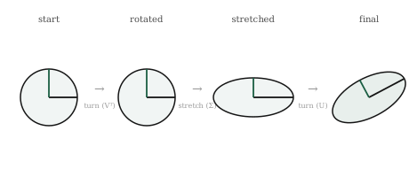
Here is the complete mathematical claim. It is worth stating plainly because it often sounds too powerful to be true. You can take any geometric transformation whatsoever. No matter how complicated its final effect on the space appears, it can always be performed in exactly three sequential steps. First, you rotate the space. Next, you stretch the space along the main horizontal and vertical axes by fixed amounts. Finally, you rotate the space a second time. Turn, stretch, turn. Every matrix is secretly just these three basic moves composed together.
We should examine why this is so remarkable. A general transformation can heavily shear the space. It can squash the space diagonally. It performs actions that seem to mix stretching and turning inseparably. This mathematical claim proves that all of that apparent complexity is simply an illusion of our viewpoint. If you rotate the space into the correct starting orientation first, the heavy action of the transformation simply becomes a basic stretch along the main axes. It becomes pure scaling with absolutely no turning. A final rotation then sets the stretched result into its correct final orientation. The apparent messiness was only caused by looking at the transformation from the wrong perspective. When you rotate into the correct frame, the math becomes incredibly simple.
Figure 11.1: Every transformation consists of three sequential moves. It applies a rotation, a stretch along perpendicular axes, and a final rotation. Every single matrix operates this exact way.
The pure stretch in the middle step is where all the valuable information lives. The numerical amounts by which this middle step stretches the axes are called the singular values of the matrix. They form the absolute heart of the decomposition. Each singular value dictates how much the transformation stretches the space along one of its special perpendicular directions. Unlike eigenvectors, these singular values are always real numbers. They are always mathematically present, and they are always ranked perfectly from largest to smallest. The largest singular value represents the strongest physical stretch of the transformation. It is the specific direction where the matrix pulls the space outward the most. The smallest singular value is simply its weakest stretch.
These singular values instantly expose the rank we defined abstractly two chapters ago. We can finally see the rank mechanically. If a transformation collapses the space, one of its stretch amounts must equal exactly zero. The middle step squashes that specific direction completely flat rather than stretching it. This means the total number of non-zero singular values perfectly equals the rank of the matrix. It is the exact number of geometric directions that survive with real mathematical reach. A massive matrix that looks completely full but secretly has a rank of two will show its true nature openly. It will have exactly two non-zero singular values, and the rest will be strictly zero. The rank we previously had to compute using complex algorithms becomes a simple property you can read straight from the stretch amounts.
This natural ranking is what makes the decomposition incredibly useful. The singular values are always ordered from strongest to weakest. They explicitly tell us which directions carry the vast majority of the transformation and which directions barely matter at all. A direction stretched enormously is performing most of the mathematical work. A direction stretched by almost nothing is practically irrelevant. If you keep the few strongest stretches and intentionally discard the rest, you create an approximation of the transformation. This approximation captures nearly all of the original effect using only a tiny fraction of the original information. This single concept of keeping the large stretches and dropping the small ones is the primary engine driving data compression and dimensionality reduction.
The math, built up
The three physical moves of turn, stretch, and turn translate into three separate matrices multiplied together. Because each individual move is a transformation, doing them in sequence is a geometric composition. This means any given matrix \(A\) can be written exactly as:
\[A = U \Sigma V^{T}\]
The three mathematical factors are exactly the three physical moves. We must read them from right to left as the rules of composition strictly demand. The rightmost factor \(V^{T}\) represents the first rotation. It turns the space directly into the correct starting frame. The middle factor \(\Sigma\) represents the pure stretch. It is a particularly simple kind of matrix. It contains zeros everywhere except straight along its main diagonal. Those diagonal entries are the singular values, providing the exact stretch amounts. The leftmost factor \(U\) represents the final rotation. It takes the newly stretched result and turns it into its final physical orientation.
Each mathematical piece carries a very clean meaning built entirely from concepts we already know. The vertical columns of \(V\) represent the special input directions. This is the perpendicular set of arrows that the first rotation perfectly aligns with the main axes. They are the specific directions the transformation treats in the simplest way possible. The columns of \(U\) show exactly where those specific directions end up pointing after the entire transformation completes. They are the final output directions. The matrix \(\Sigma\) securely holds the singular values along its diagonal in strict descending order. Each singular value pairs a specific input direction from \(V\) with a matching output direction in \(U\). It records exactly how much that specific direction is stretched during the journey between them. The entire transformation is incredibly logical. It lines up the special input directions with the axes, stretches each one by its singular value, and rotates them directly into the final output directions.
The two rotation matrices \(U\) and \(V\) possess a very special property. This property is exactly what guarantees they act as pure rotations with no accidental stretching. Their columns consist entirely of perpendicular unit vectors. This means the directions sit at perfect right angles to one another, and every single column has a physical length of exactly one. A matrix built entirely from perpendicular unit vectors is called an orthogonal matrix. An orthogonal transformation creates a perfectly rigid motion. It turns the space without stretching or squashing any part of it, permanently preserving all original lengths and internal angles. This guarantees the only stretching in the entire decomposition is strictly quarantined inside the middle factor \(\Sigma\). The two outer matrices only turn the space. The middle diagonal matrix only stretches the space. Absolutely nothing else happens mathematically.
We will not explain how these three specific factors are computed from scratch. Calculating them requires highly involved numerical algorithms. This calculation is always performed by a computer and practically never by hand for any real-world matrix. The most important detail is what the decomposition actually guarantees. It guarantees that this structure exists for every single matrix without exception. It guarantees that the singular values are always real numbers. It guarantees they are perfectly ordered and reliably expose the true rank of the data. Finally, it guarantees the entire complex behavior of the transformation is laid out clearly as a turn, a stretch, and a final turn. Those stretches are always ranked from most important to least important. That mathematical guarantee is what the rest of the chapter puts into practical action.
Build it yourself
Python using NumPy computes this entire decomposition in one simple function call. We can write code to confirm that it successfully rebuilds the original matrix. We can also verify that the singular values behave exactly as we claimed.
We will take a simple matrix and physically decompose it:
The singular values correctly come back in S, automatically ordered from largest to smallest. The arrays U and Vt represent the two rotations. They hold the output directions and the transposed input directions. You should notice that S is returned as a simple list of the singular values rather than the full diagonal matrix. Storing all the surrounding zeros in memory would be highly wasteful for large datasets. We can easily rebuild the proper diagonal matrix whenever we actually need it.
We must confirm that these three separate moves truly reassemble the original transformation. We place the isolated singular values onto a standard diagonal matrix. Then we multiply the three factors back together to execute the turn, stretch, and final turn:
Sigma = np.diag(S)reconstructed = U @ Sigma @ Vtprint(reconstructed)print(np.allclose(reconstructed, A))
[[3. 1.]
 [1. 3.]]
True
The matrix product perfectly returns the original starting matrix. The np.allclose function verifies they are identical, safely allowing for the tiny floating-point decimals these computer processors always generate. The three simple composed moves perfectly recreate the exact matrix we started with.
Now we can watch the singular values directly expose the matrix rank. We will build a matrix that secretly collapses the space. Its second column will be exactly twice the first column:
One singular value is a substantial number. The other is practically zero. It is just a tiny speck of floating-point dust sitting exactly where a true zero belongs. Having only one non-zero stretch means the matrix has a rank of exactly one. The transformation stretches a single direction and completely squashes the other one flat. This is the exact mathematical collapse we detected earlier using the determinant and the rank formulas. We can now see it visually as a stretch amount that completely fell to zero. The singular values detect the collapse exactly the same way every other tool does.
Finally, we can experience a basic version of data compression. We will intentionally keep the strong stretch and actively discard the weak one. We will take a fresh matrix, decompose it, and carefully rebuild it using only its largest singular value. We will throw the smaller stretch completely away:
A = np.array([[4.0, 1.0], [2.0, 3.0]])U, S, Vt = np.linalg.svd(A)# keep only the largest singular value, zero the restS_approx = S.copy()S_approx[1:] =0approx = U @ np.diag(S_approx) @ Vtprint("original:\n", A)print("rank-1 approximation:\n", approx)
The new approximation is not perfectly identical to the original matrix. However, it is a highly recognizable shadow of it. We successfully rebuilt it from a fraction of the total information by keeping only the absolute strongest stretch. On a tiny two-by-two matrix, the memory saving is completely trivial. However, applying this exact same move to a massive matrix is incredibly powerful. Keeping a handful of the strongest stretches out of thousands of possibilities is the exact mechanism used to compress digital images and huge datasets. The strong mathematical directions carry the primary picture. The weak directions are just minor details we can easily afford to lose.
Where it lives in ML
The singular value decomposition is one of the most heavily utilized tools in all of applied machine learning. The fundamental move it enables is keeping the strong stretches and discarding the weak ones. This capability is exactly what massive segments of the field desperately require.
We can finally explain principal component analysis properly. We have referenced this technique since the chapter on mathematical independence. PCA takes a massive cloud of scattered data, finds the specific directions along which it varies the most, and actively keeps only those vital directions. Those core directions are simply the top singular directions of the raw data. The amount the data varies along each line is provided directly by the singular values. PCA is essentially just an SVD of the data where the smallest singular values are intentionally thrown away. This explains why it can flawlessly reduce a thousand features down to a manageable handful while losing practically nothing. The discarded directions were simply the ones the data barely even used.
Data compression relies on the exact same logic. It simply applies the math to a single media object rather than an entire dataset. A digital image is just a massive grid of numbers. Because it is a grid, it is formally a matrix, and every matrix has a valid SVD. Most standard images contain a few very strong singular values that carry the broad visual structure. They also contain a long tail of tiny singular values carrying very fine visual details. If you keep the strongest few hundred stretches and discard the thousands of weak ones, you can easily rebuild the picture. The new image will be nearly indistinguishable from the original, but it uses a very small fraction of the original numbers. The rank-one approximation we built manually earlier was just the most basic version of this concept. Real compression algorithms keep significantly more than one stretch, but the underlying principle remains identical. The strong geometric directions represent the actual image. The weak directions are merely details you can comfortably afford to lose.
Automated recommendation systems rely heavily on this decomposition. The process looks almost magical when you observe it for the first time. Programmers arrange what every single user thought of every single catalog item into one enormous matrix. The individual users run down the side, and the items run across the top. The vast majority of this matrix is completely blank because most people have rated almost nothing in the store. Taking the SVD of that sparse, gigantic matrix uncovers a very small number of highly strong hidden directions. These are latent patterns of human taste that naturally explain most of the submitted ratings. It might reveal a heavy leaning toward a specific movie genre that no human ever manually labeled, but which naturally emerges from the mathematical stretches. Reconstructing the matrix using only its strongest singular directions magically fills in all the blank spots. It provides startlingly accurate guesses about what a user would think of a product they have never even seen. The recommendation you receive for the next movie to watch is simply an SVD quietly reconstructing a missing matrix entry in the background.
There is another highly valuable use tied closely to understanding and controlling what artificial models actually learn. The internal transformations inside a fully trained network naturally have singular values. Studying these specific values reveals exactly how the network physically stretches and compresses the data passing through its layers. It reveals precisely which directions the model heavily amplifies and which directions it permanently discards. Advanced techniques used to shrink or fine-tune massive models work strictly by keeping only the strongest singular directions of those internal transformations. It is the exact same logic of keeping the big stretches applied directly to a network’s weights rather than to the input data. The decomposition we just built is rapidly becoming a standard tool for looking deep inside models. It helps researchers decide what internal logic actually matters, which is absolutely vital for making powerful AI systems safe and computationally efficient.
Common misunderstandings
Singular values are definitely not eigenvalues. After reading the previous chapter, it is very tempting to treat these two concepts as identical. They are fundamentally different. Every single matrix possesses singular values. They are always real numbers, always non-negative, and always perfectly ordered. Conversely, only some specific matrices have real eigenvalues. Furthermore, eigenvalues can easily be negative or complex numbers. For the highly special and well-behaved matrices where both sets of numbers do exist, they align very closely. This alignment is exactly why the two concepts frequently get confused. The singular value decomposition functions reliably on absolutely every matrix precisely because singular values do not carry the mathematical fragility that eigenvalues do. When you require a tool that is strictly guaranteed to exist and behave predictably, you must reach for singular values.
The mathematical decomposition is completely exact. It is very easy to incorrectly assume the SVD is just an approximation method. This happens because we frequently use it to build approximations by dropping the small singular values. However, the full underlying decomposition is perfectly exact. If you keep every single singular value, the three moves multiply backward to form the precise original matrix. It is perfectly accurate to the final decimal digit the processor allows. Building the approximation is a completely separate and entirely optional second step. That step intentionally throws away the weak stretches on purpose. The raw decomposition itself hides absolutely nothing and loses zero data. Only the deliberate truncation process causes data loss.
Small singular values are not always useless noise. The concept of keeping the strong directions and dropping the weak ones is highly powerful. However, it relies heavily on one major assumption. It assumes that the weak directions carry almost nothing of value. This is usually true, but occasionally it is horribly false. In some highly specific problems, the absolute smallest singular values carry the exact subtle signal you desperately care about. Discarding them blindly throws away the entire answer. Truncating a matrix requires a human judgment call about your specific data. It is never a blind mechanical rule. This is the exact same lesson we encountered with cosine similarity and mathematical norms. The formula cannot decide if the data it removes was actually worth keeping.
A matrix is not literally built from three separate matrices. The decomposition writes \(A\) strictly as a mathematical product of three distinct factors. However, \(A\) remains one single cohesive geometric transformation. The three factors are simply a method of visualizing the movement as a turn, a stretch, and a final turn. It is not a claim that the matrix was secretly manufactured from three completely separate parts. This directly relates to a fact from the composition chapter. We previously noted that you generally cannot recover the two matrices that were combined to create a product. The SVD acts as the remarkable mathematical exception. For this specific type of factorization into three distinct pieces, there is a standard and universally correct answer. It is always mathematically available, which is exactly what makes the technique so incredibly valuable. Composition usually completely hides its original factors. The SVD is the one place where they can always be reliably recovered.
Check your intuition
Try to answer these questions before opening the answers below.
1. In the decomposition \(A = U\Sigma V^{T}\), which factor holds the stretch amounts, and which two are pure rotations?
2. A matrix has singular values \(5\), \(3\), and \(0\). What is its rank, and what does the zero tell you about the transformation?
3. Every matrix has a singular value decomposition, but not every matrix has real eigenvectors. Why is this a reason to prefer singular values for general work?
4. You compress an image by keeping only its ten largest singular values out of five hundred. What have you kept, and what have you thrown away?
5. A transformation’s singular values are \(10\), \(9.8\), \(9.5\), and \(0.01\). Which direction could you discard with the least loss, and what does the spread of values suggest about the data?
TipAnswers
1. The middle factor \(\Sigma\) holds the physical stretch amounts. It stores the singular values securely along its main diagonal with zeros everywhere else. The two outer factors, \(U\) and \(V^{T}\), are the pure mathematical rotations. The \(V^{T}\) matrix turns the space cleanly into the correct starting frame. The \(U\) matrix turns the newly stretched result directly into its final geometric orientation. All the heavy stretching is quarantined tightly in the middle. The outer two matrices only turn the space.
2. The rank is exactly two. This is simply the total number of non-zero singular values. The zero singular value proves the transformation completely squashes one specific direction flat rather than stretching it. It collapses that dimension down to absolutely nothing. This means the transformation is rank-deficient, perfectly singular, mathematically non-invertible, and possesses a zero determinant. We have gathered all these faces of a structural collapse, and they are now shown visually as a stretch amount that plummeted perfectly to zero. Exactly two geometric directions survive with real reach, and the third is completely destroyed.
3. A mathematical tool that always exists and always behaves predictably is far safer to build upon than one that frequently fails. Eigenvectors can easily output complex numbers or completely fail to point anywhere in real space. Their stretch factors do not reliably rank the importance of directions for general matrices. Conversely, singular values are always real numbers. They are always mathematically present, and they are always perfectly ordered from strongest to weakest for absolutely every matrix without exception. For general programming work, you cannot guarantee your matrix fits the well-behaved format eigenvectors demand. The singular value decomposition provides the exact geometric structure you want without carrying any of the mathematical fragility.
4. You have actively kept the ten absolute strongest stretches. These are the core directions along which the physical image varies the most. They carry the broad structural outline and the vast majority of its recognizable visual content. You have intentionally thrown away four hundred and ninety very weak directions. These contained the tiny fine details the image barely even used. The final result is a highly recognizable version of the picture successfully rebuilt from a tiny fraction of the original numbers. It remains sharp enough to see clearly even though most of the data is completely gone. The strong directions essentially formed the picture, while the discarded ones were just expendable details.
5. You could easily discard the fourth direction associated with the \(0.01\) singular value with almost zero physical loss. The transformation barely stretches it at all, so it carries almost nothing of mathematical value. The overall spread is highly telling. You have three large singular values clustered tightly together, followed by a sudden massive drop to nearly zero. This proves the data is essentially three-dimensional. It spreads richly through three core directions but remains almost completely flat in the fourth direction. This sharp cliff falling from \(9.5\) straight to \(0.01\) is the exact signature of data that lives in fewer dimensions than it initially appears to. This specific low-rank structure is what makes dimensionality reduction incredibly profitable.