import numpy as np

v = np.array([2.0, 1.0])
w = np.array([1.0, 3.0])

print(v + w)
[3. 4.]In the last chapter, we turned a single song into a vector. We visualized it as a fixed arrow in space and learned how to measure its length. That gives us a great way to talk about one song at a time. But we rarely care about just one song in the real world.
Think about what a playlist actually represents. It is more than just a list of tracks. It represents a region, a specific mood, or a stretch of space where similar songs naturally cluster together. A musical genre works exactly the same way on a larger scale. When we say two playlists overlap, or that a new track sits somewhere between two different artists, we are talking about moving through space. A single fixed arrow cannot capture that movement.
This chapter focuses on what happens when we use multiple vectors at once. If we have a handful of songs, we want to know what other music we can describe using only those initial tracks. We will explore how to build a point sitting halfway between two songs. We will see how to take a musical direction we like and follow it further than any single track goes. We will also look at how two or three vectors can map out an entirely new region of possibilities.
Everything we want to do relies on just two basic operations. We can add vectors together, and we can scale a vector up or down. Every concept in this chapter is built entirely from these two actions. They are simple enough to define in a single sentence, yet they form the foundation of almost everything linear algebra accomplishes.
Let us start with adding vectors. We established earlier that a vector is a journey rather than a fixed destination. The vector \([3, 4]\) means moving three steps across and four steps up. It only ends on a specific coordinate because we chose to start at the origin. Since a vector is a set of movements, adding two of them together is straightforward. You simply complete the first journey, and then start the second journey from wherever the first one left you.
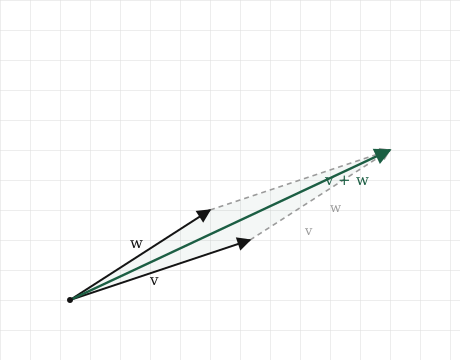
Picture two vectors named \(\mathbf{v}\) and \(\mathbf{w}\). First, walk along \(\mathbf{v}\) from the origin to its tip. Then, without returning to the start, walk along \(\mathbf{w}\) beginning right where \(\mathbf{v}\) ended. You will finish in a completely new location. If you draw a fresh arrow from the original starting point straight to this final destination, that new arrow represents the sum \(\mathbf{v} + \mathbf{w}\). When you lay the vectors out end to end like this, the visual result makes perfect sense.
The order of the journeys does not matter at all. If you walk \(\mathbf{w}\) first and then follow with \(\mathbf{v}\), you will land in the exact same spot. You simply trace the opposite sides of a parallelogram. Two vectors and their sum will always form this specific four-sided shape. Keep this visual in mind moving forward. Adding vectors creates a parallelogram, and their sum points directly to the far opposite corner.
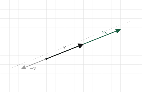
Scaling is the second operation, and it is even simpler. To scale a vector, you just stretch it or shrink it. If \(\mathbf{v}\) is a specific journey, then \(2\mathbf{v}\) means walking twice as far in the exact same direction. Similarly, \(\tfrac{1}{2}\mathbf{v}\) means walking half the distance. The arrow never changes its angle. Scaling only impacts the length of the vector without ever turning it.
There is one special case you should know about. Scaling by a negative number like \(-1\) might seem strange at first, but it follows the same logic. The arrow stays on its original path, but it flips to point backward along that line toward the far side of the origin. Negative scaling still respects the original path. It simply travels the exact same line in the reverse direction.
Now we can put these two actions together to unlock the real power of this chapter. We can take two vectors, scale each one by any amount we choose, and then add the results together. This creates an equation like \(2\mathbf{v} + 3\mathbf{w}\) or \(\tfrac{1}{2}\mathbf{v} - \mathbf{w}\). Taking a specific amount of one vector and adding it to a specific amount of another is called a linear combination. This is easily the most important mathematical concept in this section of the book. Almost everything we do later will just be a linear combination in a slightly different format.
Mastering linear combinations naturally leads us to a fascinating question. If we are allowed to use every possible combination of \(\mathbf{v}\) and \(\mathbf{w}\), including all positive, negative, and fractional amounts, where can we actually travel? The complete set of every destination we can reach is called the span of those two vectors. Picturing how span works is our next step.
We now understand adding and scaling as visual pictures. To teach a computer to do this work, we have to translate those pictures into arithmetic. Fortunately, the math for both operations is incredibly basic.
Let us look at addition first. Assume we have a vector \(\mathbf{v} = [v_1, v_2]\) and another vector \(\mathbf{w} = [w_1, w_2]\). We want to find the single arrow that represents walking \(\mathbf{v}\) followed by walking \(\mathbf{w}\). The first vector moves us \(v_1\) steps across and \(v_2\) steps up. The second vector moves us an additional \(w_1\) steps across and \(w_2\) steps up. To find the total journey, we simply add the horizontal steps together and the vertical steps together.
\[ \mathbf{v} + \mathbf{w} = [v_1 + w_1, \; v_2 + w_2] \]
That is the entire rule for vector addition. You add vectors together by combining the numbers that sit in matching slots. You add the first number to the first number, and the second to the second. The visual drawing of placing vectors end to end matches this arithmetic perfectly. The drawing is what our eyes see, and the arithmetic is what the machine computes.
The math for scaling is even faster. If you want to walk twice as far along vector \(\mathbf{v}\), you double every step in the list. To scale the vector by any generic amount \(c\), you just multiply every number by \(c\):
\[ c\,\mathbf{v} = [c\,v_1, \; c\,v_2] \]
You just multiply every single number in the list by your chosen scale factor. That covers everything you need to know about scaling. You can also see how negative scaling works without needing a special rule. Setting \(c = -1\) simply multiplies each number by negative one. This mathematically flips the arrow to the opposite side of the origin, perfectly matching our earlier visual drawing.
These two operations work perfectly on much longer lists without changing the underlying idea. If you have a vector with three hundred numbers, you still add them slot by slot using three hundred small addition problems. You scale that large vector by multiplying all three hundred numbers by your scale factor. The rule stays exactly the same no matter how long the list gets. This consistent pattern will guide us through the entire book.
Now we can formally define the main concept of this chapter. If you scale several vectors and add the results together, you create a standard recipe:
\[ c_1 \mathbf{v}_1 + c_2 \mathbf{v}_2 + \cdots + c_k \mathbf{v}_k \]
This formula represents a linear combination of the vectors \(\mathbf{v}_1\) through \(\mathbf{v}_k\). The numbers \(c_1\) through \(c_k\) represent the scaling amount for each specific vector. These amounts can be any number you like, including positive integers, fractions, negative values, or even zero. A linear combination simply takes our two basic operations, applies them at the same time, and produces one final resulting arrow.
The fact that the scaling amounts can be anything is highly important. This freedom allows us to explore a massive continuous region of space rather than just pointing at a few disconnected spots. Imagine fixing two base vectors named \(\mathbf{v}\) and \(\mathbf{w}\). If we let their scaling amounts sweep through every possible pair of numbers, we can build an endless number of new arrows. The complete collection of all these possible destinations is called the span of those two original vectors.
When two vectors point in distinctly different directions, their span covers the entire flat plane. You can reach any coordinate on the page by walking a specific amount along \(\mathbf{v}\) and a specific amount along \(\mathbf{w}\). By carefully adjusting the scale of each vector, you can steer your way to absolutely any location.
These operations are simple to do on paper. They are even easier to perform in Python using NumPy. The concept of adding things slot by slot is naturally built into how NumPy handles arrays.
Let us start by defining two vectors and adding them together:
import numpy as np
v = np.array([2.0, 1.0])
w = np.array([1.0, 3.0])
print(v + w)[3. 4.]The program outputs [3.0, 4.0]. This happens because it adds the first numbers together to get three, and the second numbers together to get four. Notice that we did not have to write a loop or tell the computer to handle the numbers one at a time. We just wrote v + w, and NumPy automatically matched each slot with its partner. The slot-by-slot addition rule is hardwired directly into the plus symbol.
Scaling works exactly the same way. When you multiply a vector by a normal number, the program updates every slot in the list instantly:
print(2 * v)
print(0.5 * v)
print(-1 * v)
[4. 2.]
[1. 0.5]
[-2. -1.]We just performed three different scalings without a single loop. Writing 2 * v doubles every number in the list. Writing 0.5 * v cuts the numbers in half. Writing -1 * v flips the positive values to negative values, drawing the arrow pointing backward through the origin.
Now we can combine both actions into a linear combination. We will write code for \(2\mathbf{v} + 3\mathbf{w}\):
print(2 * v + 3 * w)[ 7. 11.]That single line of code instructed the computer to scale two separate vectors and add the final results together. NumPy reads the math exactly how a human does. It handles the scaling first, and then it performs the addition. Every linear combination you will ever write in code will follow this exact pattern. You just add more vectors to the line.
It is a good idea to verify that NumPy is truly following our slot-by-slot rule without doing anything unexpected. We can spell out the math manually, build a new list one position at a time, and compare the result against the built-in addition:
by_hand = np.array([v[0] + w[0], v[1] + w[1]])

print(by_hand)
print(v + w)
print(np.array_equal(by_hand, v + w))
[3. 4.]
[3. 4.]
TrueThe version we built by hand matches v + w perfectly. The np.array_equal function confirms they are identical. There is no hidden magic in the plus symbol. It is just applying our basic math rule to every slot.
We should highlight one final important detail about scaling and adding. Just like measuring length, these operations do not care how many numbers live in your vector. If you use vectors with three hundred numbers, every line of code above still runs perfectly. The v + w command will add all three hundred slots in an instant. Writing 2 * v will scale all three hundred numbers simultaneously. A linear combination handles massive datasets without requiring a single change to the code. Our visual drawings fail after three dimensions, but the arithmetic and the Python code keep working flawlessly.
Adding and scaling might seem too basic to be useful in advanced programming. But these simple actions are actually the foundation of the entire field. Nearly every calculation a neural network performs is built on linear combinations.
Consider a single artificial neuron, which is the fundamental building block of a machine learning network. A neuron receives a set of numbers from previous neurons in the form of a vector. It also holds its own internal vector of the same length, which we call its weights. To calculate an answer, the neuron multiplies each incoming number by its corresponding weight and adds the total together. This multiplying and adding process is exactly what a linear combination is. The weights simply act as the scaling amounts. You can think of a neuron as a linear combination that has learned an opinion about which incoming numbers are the most important.
A layer in a network is just a large group of these neurons working at the same time. This means a single layer is just running many linear combinations on the same input data, with each neuron using its own unique weights. A full network is just many of these layers stacked on top of each other. The vast majority of a trained model is just linear combinations repeating over and over at a massive scale. When a company announces a new model with seven billion parameters, they are primarily just counting the scaling amounts inside millions of linear combinations.
Because these fundamental operations are so reliable, we can actually perform arithmetic on abstract concepts. Remember that a computer understands a word as a vector containing a few hundred learned numbers. Researchers discovered that you can add and subtract these word vectors, and the mathematical result will point to a related word. A famous example involves royal titles:
\[ \text{king} - \text{man} + \text{woman} \approx \text{queen} \]
If we treat the words as vectors, this equation is just basic addition and scaling. You start at the vector for the word king. You subtract the vector for man, which is the same as scaling it by negative one and adding it. Then you add the vector for woman. The final resulting arrow points directly at the coordinates for the word queen. The spatial distance between man and woman is mathematically parallel to the distance between king and queen. No programmer hardcoded this relationship. The model discovered the geometry of language completely on its own, and we can navigate that geometry using the simple math from this chapter.
We also need to understand a very important limitation of this math. Because a linear combination only uses scaling and adding, it can never perform more complex geometric transformations. Scaling and adding can stretch a space, slide it around, and even flip it backward. However, these operations can never bend or curve the space. If you stack a hundred layers that only use linear combinations, the entire massive network is still restricted to straight lines. It would never be able to separate complex, tangled data sets because stretching and sliding is not enough. This strict adherence to straight lines is exactly what the word linear means. It is the defining feature of linear algebra.
Earlier we mentioned that neurons take one small extra step after running their linear combination. That step is far more than a minor detail. The extra step introduces a mathematical bend into the data. That curve is the only reason stacking multiple layers makes a neural network smarter. Without that bend, the entire deep network would mathematically collapse back into a single basic linear combination. We will explore how to build that bend when we dive deep into neural networks in Part 4. For now, simply remember that linear combinations act as the main engine for the entire machine learning process.
Span does not always fill the entire space. We established earlier that the span of two vectors typically covers a whole flat plane. That is usually true, but there is an important exception. Imagine two vectors that point along the exact same visual line, like \(\mathbf{v} = [1, 1]\) and \(\mathbf{w} = [2, 2]\). The second vector is just the first vector multiplied by two. It does not introduce any new direction into the math. No matter how you combine or scale these two specific vectors, your final destination will always be trapped on that single straight line. The overall span shrinks from a wide plane into a narrow path. Two vectors can only fill a plane if they bring distinct, independent directions to the table. If one is just a scaled copy of another, they cannot escape their single line.
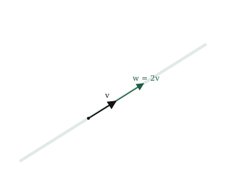
This collapsing span is an important problem to watch out for. It is the reason we will soon introduce complex terms like independence and rank. Asking whether our vectors offer genuinely different directions or if some of them are just redundant copies is a critical part of machine learning. We will learn how to measure this precisely in the next few chapters.
Scaling with negative numbers is different from subtraction. It is easy to look at \(-2\mathbf{v}\) and think it means subtracting two copies of the vector. That implies we are taking something away, which is incorrect. Scaling a vector by negative two creates a brand new arrow. This new arrow is twice as long and points in the complete opposite direction. Subtraction only happens when you take that new, negatively scaled arrow and add it to a different vector. You should treat scaling as a way to reshape a single arrow, while subtraction is a process of combining two different arrows together.
Adding vectors is not the same as averaging them. When you add two vectors together, your final arrow lands at the far corner of the parallelogram. This point is pushed much further outward than either starting vector. Addition does not find the middle ground between two things. Finding a midpoint requires a specific linear combination where both scaling amounts are set to exactly one half. Basic addition and averaging might feel conceptually similar, but mathematically they send you to entirely different coordinates.
Length does not equal importance. It is incredibly common to assume that the longest vector in a linear combination is the most important one. This is a false assumption. The raw length of an arrow and its actual influence in the calculation are completely separate things. A very short vector scaled by a massive amount will have a huge impact on the final result. A massive vector scaled by a tiny fraction will barely register. The influence of a vector is determined entirely by its scaling amount rather than its starting physical length.
Try to solve these problems before reading the answers. These questions will test how well you understand the concepts rather than asking you to memorize basic rules.
1. We have \(\mathbf{v} = [2, 1]\) and \(\mathbf{w} = [1, 2]\). What is \(\mathbf{v} + \mathbf{w}\), and what is \(\mathbf{v} - \mathbf{w}\)? Try drawing both to help visualize the math.
2. Take a single vector \(\mathbf{v} = [3, 1]\). Describe the complete set of points you can reach using only scalings of \(\mathbf{v}\). What shape does this set create?
3. We have two vectors \(\mathbf{v} = [1, 0]\) and \(\mathbf{w} = [2, 0]\). Can we reach the point \([0, 1]\) by combining them? Why or why not?
4. Find the scaling amounts \(a\) and \(b\) that make \(a\,[1, 0] + b\,[0, 1]\) equal to \([5, 3]\). Now try to do the same thing for any general target \([x, y]\).
5. Is the midpoint between \(\mathbf{v}\) and \(\mathbf{w}\) considered a linear combination of those vectors? If so, what are the two scaling amounts?
1. By adding slot by slot, we get \(\mathbf{v} + \mathbf{w} = [3, 3]\). By subtracting, we get \(\mathbf{v} - \mathbf{w} = [1, -1]\). The combined sum leans up and to the right, finding a new direction between the two originals. The subtracted difference points down and to the right. Subtraction is essentially just adding a negatively scaled vector, which is why the resulting arrow swings below the axis.
2. Every possible scaling of this vector takes the form \([3c, \; c]\), where \(c\) represents any positive, negative, or zero amount. As you sweep through every possible value for \(c\), you trace a straight line passing directly through the origin along the vector’s specific angle. The shape is simply a straight line. This proves that a single vector spans exactly one line.
3. No, it is impossible. Both \(\mathbf{v}\) and \(\mathbf{w}\) have a second number of zero. Any combination of these vectors will always result in a second slot equal to zero. The target point \([0, 1]\) has a one in the second slot, making it permanently out of reach. These two vectors point the exact same way and only map out a horizontal line.
4. To reach \([5, 3]\), we need \(a = 5\) and \(b = 3\). For a general target of \([x, y]\), you simply set \(a = x\) and \(b = y\). These specific base vectors are very special because the required scaling amounts are identical to the target’s own coordinates. This is a crucial concept regarding reference vectors that we will explore more deeply later.
5. Yes, the midpoint is a linear combination. The formula is \(\tfrac{1}{2}\mathbf{v} + \tfrac{1}{2}\mathbf{w}\). Both scaling amounts are exactly one half. This pulls the final arrow tip directly back to the middle space, which is exactly what an average is designed to do.