import numpy as np

v = np.array([3.0, 4.0])
print(v)
[3. 4.]Imagine you are listening to a streaming service, and a song comes on that perfectly matches your mood. The system chose that track for you, but it obviously has no concept of what music actually is. It has never felt a beat or had a chorus stuck in its head. It simply ran a calculation.
To the computer, comparing two songs is an entirely mechanical process. It needs a reliable, step-by-step way to measure similarity. This brings us to the core question of this chapter:
What do we have to turn a song into so that a machine can measure how close it is to another song?
The machine does not need to understand the music or appreciate the artist. It just needs a mathematical format that allows it to pull out numbers, compare them, and make a decision. Turning real-world items into measurable numbers is the very first step in all of machine learning. Every recommendation you receive, every facial recognition unlock, and every auto-completed sentence starts right here.
Let us take a single song and pretend there are only two things we can measure about it. We will use tempo and loudness. We can write each property down as a number, turning the song into a pair like 128 and 7.
That pair of numbers is called a list, and the order is incredibly important. We have to agree that tempo always comes first and loudness comes second. Without a fixed rule, the numbers lose their meaning entirely.
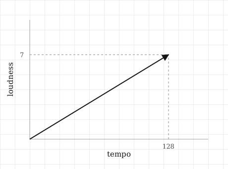
Now let us draw this song on a page. We can put tempo on a horizontal axis and loudness on a vertical one. Starting from the corner where the axes meet, we move 128 steps to the right and 7 steps up, and we make a mark. If we draw an arrow from the starting corner to that mark, we have just turned our two numbers into a physical shape.
This arrow gives us two specific properties. It points in a certain direction, and it has a specific length. Both of these properties came directly from our original two numbers. If you walk the same steps again, you will land in the exact same place every single time.
Here is the central idea we will build on. The list and the arrow are the exact same object looked at in two different ways. The list tells us how far to travel along each axis, and the arrow shows us where that journey ends. We keep both representations because each one solves a different problem. The list is perfect for a computer because a machine only knows how to process numbers in memory. The arrow is helpful for us because human beings are highly visual, and we can easily see if two arrows point in the same direction.
Two details are worth pinning down before we move on.
First, the order of the numbers is a strict rule. If we swap them to 7 and 128, we describe a song crawling at 7 beats per minute at a deafening volume. The slots carry meaning, so moving a number changes everything.
Second, this concept does not stop at two numbers. If we add a third number for danceability, our arrow moves off the flat page and into a 3D room. If we add a fourth number, our eyes can no longer picture the arrow at all. But the computer does not mind in the slightest. The list simply gets longer. Everything we build will keep working in those higher spaces we cannot see, which is where real machine learning data actually lives. A real song on Spotify is not just two numbers, but hundreds of them.
So let us return to our original problem. Two songs become two arrows. When the songs are similar, their arrows point in roughly the same direction. When they share nothing in common, they point away from each other. Measuring how closely two arrows align gives us a numerical answer, which is exactly what the machine needs to make a recommendation.
The mathematical name for this list that doubles as an arrow is a vector. Every vector in this book is exactly what we just built. It is a set of numbers sitting in fixed slots, which we can also visualize as an arrow.
To work with a vector, we need a standard way to write it down. We give it a name and place its list in brackets:
\[ \mathbf{v} = [128, 7] \]
The name \(\mathbf{v}\) is written in bold so we know it represents a whole vector and not just a single number. The brackets hold the list itself. This notation is universal, so once you get comfortable reading it here, you will recognize it in any other technical text.
With this notation ready, we can ask our first mathematical question. How long is that arrow?
Let us look at the drawing again. The arrow and the two dashed lines reaching down to the axes form a right-angled triangle. The dashed lines are the short sides, which measure 128 and 7. The arrow is the long side.
You likely remember how to find the long side of a right-angled triangle from school geometry. You square the two short sides, add them together, and take the square root. This is the Pythagorean theorem, and it directly gives us the length of our vector:
\[ \lVert \mathbf{v} \rVert = \sqrt{v_1^2 + v_2^2} \]
We read the left side as the length of \(\mathbf{v}\). We use double bars to show we are measuring the size of a whole vector, compared to the single bars \(|x|\) used for ordinary numbers. On the right side, \(v_1\) is the first number in the list and \(v_2\) is the second. We are simply letting the math handle what we could otherwise measure with a physical ruler.
Let us check this with a simple vector like \(\mathbf{v} = [3, 4]\):
\[ \lVert \mathbf{v} \rVert = \sqrt{3^2 + 4^2} = \sqrt{9 + 16} = \sqrt{25} = 5 \]
The length is exactly five. The formula allows a machine to figure this out without needing to analyze an image.
Now imagine we add a third number to make the vector \([v_1, v_2, v_3]\). The formula keeps the exact same shape:
\[ \lVert \mathbf{v} \rVert = \sqrt{v_1^2 + v_2^2 + v_3^2} \]
It does not matter if we have three numbers, four numbers, or three hundred numbers. You just keep squaring, adding, and taking the root:
\[ \lVert \mathbf{v} \rVert = \sqrt{v_1^2 + v_2^2 + \cdots + v_n^2} \]
This is a crucial moment to pause. Our human ability to visualize runs out after three dimensions. The math does not. The formula just keeps processing the numbers and hands back a value that behaves exactly like a physical length. By turning the picture into arithmetic, we are free to explore spaces our eyes cannot follow.
We have found a way to extract a single number from a single song. But to compare two songs, we need a way to take two vectors and get a single number back that tells us how closely they align. That will be our next step.
We have found the length of an arrow manually, but the goal is to let a computer do the heavy lifting. Let us build the exact same process in Python using NumPy.
First, we define the vector:
import numpy as np
v = np.array([3.0, 4.0])
print(v)[3. 4.]Notice what we gave the computer. We simply handed it a list of two numbers. The machine has no concept of the visual arrow, but the raw numbers are all it actually needs.
Now we can compute the length exactly as the formula dictates. We square each number, add them together, and take the square root:
squared = v ** 2
total = np.sum(squared)
length = np.sqrt(total)

print(squared)
print(total)
print(length)
[ 9. 16.]
25.0
5.0We just performed the arithmetic step by step. The squares are 9 and 16, they add up to 25, and the root is 5.0.
NumPy also gives us a built-in function to handle this entire process at once:
print(np.linalg.norm(v))5.0The word norm is just the formal mathematical term for length. This function does exactly what we did manually a moment ago. We can even ask Python to confirm that both methods return the identical result:
print(np.sqrt(np.sum(v ** 2)) == np.linalg.norm(v))TrueThe result is True, proving the built-in library is just a convenient shortcut for our basic formula.
Now we can test the real power of this concept. Let us create a vector with three hundred numbers, simulating a more realistic dataset:
rng = np.random.default_rng(0)
big = rng.random(300)

print(big.shape)
print(np.linalg.norm(big))
(300,)
10.683214066915752The machine returns a length instantly. This highlights the entire point of the chapter. We asked for the length of a 300-dimensional arrow, an object completely impossible to visualize. The computer solved it in milliseconds using the exact same triangle math we learned in geometry. The underlying code never changes or needs special rules for higher dimensions. In practice, you will only ever write the np.linalg.norm function, but you now know exactly what is happening under the surface.
Every piece of data a machine learning model learns from arrives as a vector. It is simply the only format a machine can process.
A house prediction model sees a house as a vector. Three bedrooms, ninety square meters, and a build year of 1974 becomes \([3, 90, 1974]\). The model does not see a neighborhood or afternoon light through a window. It only sees the list.
An image is also a vector. We read the brightness of every pixel in a specific order and lay the values end to end. A photograph turns into a list of hundreds of thousands of numbers. Words are vectors too, though they are a bit more abstract. Since a word like “coffee” has no natural measurements to read, a model learns to invent numbers based on context. It figures out that “coffee” should sit close to “tea” and far away from “bulldozer” in our vector space. None of these generated numbers mean anything individually. It is the overall shape and location of the list that matters.
In all of these cases, a human had to decide what information goes into which slot. This setup process is rarely a quick step. It is often the most time-consuming part of any machine learning project.
So where is calculating the length of a vector actually useful? There are two main places we will explore properly later.
The first is normalising. If we divide a vector by its own length, we shrink or stretch it so it is exactly one unit long while still pointing in the same direction. This lets us compare the pure direction of two items without getting distracted by their raw size.
The second use is gradient clipping. When a model trains itself, the correction signals it uses are vectors. Sometimes the length of these correction vectors grows dangerously out of control. We measure the length constantly to catch these spikes, scaling them back before they break the learning process.
Now we need to discuss how this math can quietly fail.
The most obvious mistake is putting numbers in the wrong slots. If you put tempo first for some songs and loudness first for others, the math will run perfectly but your distances will be complete nonsense. The machine will not warn you because the lists still look mathematically valid.
A more subtle failure happens with scale. Look back at our song \([128, 7]\). Tempo lives in the hundreds while loudness is in single digits. When we square them for the length formula, we compare 16,384 against 49. Tempo was originally eighteen times larger, but squaring stretches that gap dramatically into a factor of over three hundred. The final length value will be entirely dominated by the tempo, while the loudness is basically ignored.
The math did exactly what we asked. The problem is that we fed it numbers on wildly different scales, and the formula assumes all slots are equally important. Having the correct formulas is only half the battle. Understanding what the numbers represent before you calculate anything is what determines if a project will actually work.
A vector is not a point. We drew our vector as an arrow ending at three across and four up. It is tempting to think the vector is just that final coordinate point. It is not. The vector is the instruction to travel three right and four up. It only ends on that specific spot because we chose to start drawing at the origin. Start somewhere else, and you finish somewhere else. The journey itself remains identical. This distinction is vital when we start adding vectors together later.
The numbers describe the arrow, not the other way around. Our song was \([128, 7]\) when we measured tempo in beats per minute. If we switch to beats per second, the exact same song becomes \([2.13, 7]\). The underlying item has not changed at all, only our convention for describing it. If your numbers ever look wrong, check your measurement conventions before assuming the data is broken.
Avoid the strict physics definition. In a physics class, a vector is often defined as something with a magnitude and a direction, like wind speed or physical force. That is a fine visual for the physical world, but it is backward for machine learning. Here, the raw numbers come first. A word embedding has hundreds of numbers that we cannot neatly map to a physical direction. The direction and length are just secondary properties we calculate from the numbers when we happen to need them.
The machine’s arithmetic is not perfectly exact. Earlier we asked Python if our manual formula equaled the library function, and it returned True. We were slightly lucky because our numbers were clean. Computers store most numbers as very close approximations. Two different calculation routes can easily end up a tiny fraction apart. If you demand exact equality, the computer might say False for two numbers that are practically identical. A safer habit is to use the np.isclose function whenever division or square roots are involved:
print(np.isclose(np.sqrt(np.sum(v ** 2)), np.linalg.norm(v)))TrueHigher dimensions behave strangely. We spent plenty of time celebrating that our length formula works perfectly in higher dimensions. However, do not assume your human intuition translates just as easily. Three-hundred-dimensional space is not just regular space with extra room. Bizarre things happen out there. For example, if you pick two random vectors in three hundred dimensions, they will almost always be at right angles to each other. The math is fully correct, but the visual instincts you built on flat paper will fail you. This concept is called the curse of dimensionality, and we devote an entire future chapter to it.
Try to reason through these questions before expanding the answers. This is about applying the concepts rather than simply recalling formulas.
1. What does the arrow for the vector \([0, 0]\) look like? How long is it, and which way does it point?
2. We have two songs, and the numbers for the second song are exactly double the first. The first is \([60, 4]\) and the second is \([120, 8]\). How do their arrows compare if we draw them?
3. We measure two songs as \([1000, 2]\) and \([1000, 9]\). If we only look at the length of each vector, can we tell the songs apart?
4. Does the vector \([3, 4]\) have the same length as \([4, 3]\)? Are they the same vector?
5. What is the length of \([1, 1, 1, 1]\)? You will need to calculate this one since we cannot draw it.
1. The length is zero, and it has no direction at all. It is just a dot resting exactly where it started. This matters because you cannot divide by zero. That means the zero vector is the only vector we cannot normalise.
2. They point in the exact same direction, but the second arrow is simply twice as long. This introduces the concept of scaling. You can multiply every number in a vector by the same amount, and the arrow will stretch or shrink without ever changing its angle.
3. You can barely tell them apart. The length of the first is approximately 1000.002, and the second is roughly 1000.040. The songs are very different in the second slot, but that difference is completely overshadowed by the massive number in the first slot. This perfectly illustrates why mixing different scales in a vector can hide important data.
4. They share the exact same length of 5. However, they are completely different vectors. The first moves three right and four up, while the second moves four right and three up. They point in different directions and end in entirely different places.
5. The length is 2. The calculation is \(\sqrt{1^2 + 1^2 + 1^2 + 1^2} = \sqrt{4} = 2\). We get a clean, perfect answer without ever needing to visualize a four-dimensional shape.