import numpy as np

v = np.array([3.0, -4.0])

l2_by_hand = np.sqrt(np.sum(v ** 2))
print(l2_by_hand)5.0At the beginning of the book, we measured the length of an arrow using the Pythagorean theorem. We squared the numbers, added them together, took the square root, and accepted the result as the true length. That calculation remains completely valid, and nothing in this chapter will contradict it. However, that calculation relies on a quiet assumption we never actually discussed. It is important to examine this assumption now because we unknowingly made a choice about how to measure our data.
When we calculated the distance from the origin to the tip of the arrow, we measured it as a bird would fly. We drew a single straight line cutting diagonally across the space, ignoring any obstacles. That straight line is a completely valid way to measure distance, but it is not the only available method.
Consider how you navigate a city arranged in a grid of streets. You cannot cut diagonally through the solid buildings. You must walk a specific distance along one street, turn the corner, and walk another specific distance along the next street. The distance you actually travel is the sum of those two separate walks rather than the direct diagonal path. Both methods start and finish in the exact same places, yet they produce two completely different numbers for the total distance. Both numbers are mathematically correct. The bird and the pedestrian simply disagree because they are trying to answer two different questions.
This means asking how far apart two vectors are does not have a single universal answer. The result changes depending on the specific rules of travel we apply. Each set of rules creates a different formal definition of length. The straight-line calculation from the first chapter is just one member of a larger mathematical family. This chapter explores that broader family to see what the other members actually measure. We will also discover why choosing the correct measurement in machine learning is so critical, as one specific method naturally forces a model to discard data features it no longer needs.
Let us place two points on a standard grid. The first point is the origin, and the second point sits three units across and four units up. We already know how to find the straight-line distance because we performed this exact calculation earlier. The Pythagorean theorem gives \(\sqrt{3^2 + 4^2} = 5\). The bird travels a distance of exactly five.
Now imagine walking that same route as a pedestrian restricted to the streets. You move three blocks across and four blocks up. It does not matter what specific path you take or how many times you turn. Every valid route that stays on the grid will cover the exact same total distance of \(3 + 4 = 7\). The pedestrian travels a distance of seven. We have two mathematically sound distances for the same two points. The only difference is whether the rules allow us to cut directly across the open space.
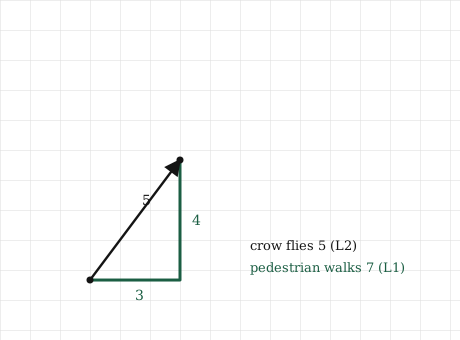
These two methods of measuring have standard technical names. The straight-line distance we learned first is called the L2 norm. The grid-based distance, where we sum our movements along each separate axis, is called the L1 norm. These specific names will make more sense when we look at the underlying equations. For now, simply remember the visual difference. The L2 norm cuts a direct path, while the L1 norm strictly follows the grid.
There is a second way to visualize this difference, and it becomes incredibly important when we reach practical machine learning. We need to ask what a distance of exactly one looks like under both sets of rules. If we collect every possible point that sits exactly one unit away from the origin, we can see what physical shape those combined points create.
Under the straight-line rules of the L2 norm, every point at a distance of one forms a perfect circle. A circle is fundamentally defined as the collection of all points sitting at a fixed straight-line distance from a central origin. This visual result matches our basic geometry perfectly.
Under the grid-based rules of the L1 norm, the resulting shape is not a circle at all. The points sitting at an L1 distance of one trace out a rigid diamond. This shape looks like a square balanced on its corner, with its tips resting directly on the main axes and its flat edges cutting diagonally across the empty space. This might seem strange until you measure the individual points. A point sitting one full step out along a single axis uses up the entire travel budget instantly. However, a point moving diagonally into the open space must spend its limited budget of one on both axes simultaneously. It cannot travel very far in either direction before running out of distance, which pulls the boundary sharply inward. This combination of reaching far along the axes and pinching inward on the diagonals creates the diamond shape.
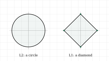
This diamond shape is an essential concept. The fact that the L1 shape has sharp points resting exactly on the axes, while the L2 shape remains perfectly smooth, might look like a minor geometric detail. It is actually a crucial mechanical difference. When we apply this to machine learning models, those sharp corners are the exact reason the L1 norm can perform tasks the L2 norm simply cannot handle. We will explain the exact mechanism shortly. For now, you only need to remember that the diamond has sharp corners on the axes, and the circle has no corners at all.
Both norms are very easy to write down as formulas. Placing them side by side shows exactly what mathematical rules they share and where their logic separates.
We can start with the calculation we already know. The L2 norm squares each individual number, adds them all together, and takes the final square root:
\[\lVert \mathbf{v} \rVert_2 = \sqrt{v_1^2 + v_2^2 + \cdots + v_n^2}\]
The only new addition here is the small number 2 tucked under the vertical bars. In the first chapter, we simply wrote \(\lVert \mathbf{v} \rVert\) without any subscript because we only had one version of length to worry about. Now that we have multiple options, the subscript tells us exactly which rule to apply. If you see the symbol without a subscript later in this book, you should always assume it means the standard L2 norm. We will only use the explicit subscripts when we need to carefully tell them apart.
The L1 norm uses an even simpler formula, and it is highly transparent about how it handles the numbers. It does not use any squares or square roots. You simply take the positive size of each number, ignoring any negative signs entirely, and add those values together:
\[\lVert \mathbf{v} \rVert_1 = \vert{}v_1\vert{} + \vert{}v_2\vert{} + \cdots + \vert{}v_n\vert{}\]
This represents the grid-based pedestrian distance translated into symbols. Each \(\vert{}v_i\vert{}\) represents the specific distance traveled along a single street, and the final norm calculates the total length of the walk. The absolute value bars ensure we measure physical distance without worrying about direction. Walking three blocks backward is still three total blocks of walking, so a negative three simply becomes a positive three in the calculation.
We should compare what these two equations have in common. Both formulas take the numbers from the list, apply a mathematical rule to remove the negative signs, and add the resulting values together. The L2 norm removes the signs by squaring the numbers, which also heavily stretches out the larger values. The L1 norm removes the signs using absolute values, which treats every single unit of distance exactly the same way. This single decision to square the numbers or leave them alone is the mathematical reason their visual shapes look so different.
The technical naming convention is also part of a larger pattern. There is a complete family of norms based on choosing a parameter called \(p\). The general rule is to raise every positive size to the power of \(p\), add them together, and then take the \(p\)-th root of the final sum. If you set \(p\) equal to 2, the formula uses squares and square roots to become the L2 norm. If you set \(p\) equal to 1, the powers basically do nothing, leaving behind the simple addition of the L1 norm. Other variations exist, but these two specific members handle almost all the heavy lifting in standard machine learning. We will not need the general equation again. You simply need to know these two calculations are closely related, and the numerical subscript tells you which one is currently active.
Both norms are very short to write in Python using NumPy. Building each calculation by hand first proves there is no hidden magic beyond the basic formulas.
We will take a small vector and compute its L2 norm manually. We square the numbers, sum them up, and take the root exactly as we learned earlier:
import numpy as np
v = np.array([3.0, -4.0])
l2_by_hand = np.sqrt(np.sum(v ** 2))
print(l2_by_hand)5.0The computer outputs a clean five, confirming the direct path. Notice that the calculation successfully ignored the negative direction because squaring the negative four automatically turned it into a positive number. Now we can compute the L1 norm manually by extracting the positive size of each number and adding them up:
l1_by_hand = np.sum(np.abs(v))
print(l1_by_hand)7.0The output is seven, which matches the pedestrian’s path. The np.abs function removes the negative sign, leaving a positive three and a positive four. The final sum is seven. We successfully generated two different distances for the exact same vector.
NumPy provides a built-in function called np.linalg.norm to handle this work. You can steer this function using an argument named ord to pick which specific norm you want. If you leave the argument blank, it defaults to the standard L2 norm:
print(np.linalg.norm(v))        # L2, the default
print(np.linalg.norm(v, 2))     # L2, asked for explicitly
print(np.linalg.norm(v, 1))     # L1
5.0
5.0
7.0The first two print commands output five. The system used the L2 calculation by default for the first line and by explicit request for the second line. The third command outputs seven. That single argument determines if the computer uses the straight path or the grid path, completely matching the numerical subscripts we discussed earlier.
We can run a quick check to prove the built-in library is strictly following our manual formulas without doing anything unexpected:
print(np.linalg.norm(v, 2) == l2_by_hand)
print(np.linalg.norm(v, 1) == l1_by_hand)
True
TrueBoth checks return True. The built-in commands simply provide a convenient shortcut for the exact mathematics we wrote out by hand.
As with all our previous operations, these calculations work perfectly on massive datasets. If you feed the computer a list of three hundred numbers, both norms calculate instantly. The ord argument simply chooses which type of distance to measure inside a high-dimensional space we cannot visually comprehend.
The two norms handle very different tasks in machine learning. The L1 norm provides a unique and highly valuable capability, which is exactly why we needed to remember its diamond shape.
Let us start with the task both norms share. A trained machine learning model relies on a massive collection of internal numbers called weights. If left unchecked, these weights naturally grow quite large during the training process. Huge weights make a model highly brittle. It memorizes the training data too tightly and fails when analyzing anything new. The standard solution is to add a mathematical penalty that punishes the model for growing large weights. This pushes the system to keep the numbers as small as possible while it learns. The overall size of the weights is measured using a norm, and your choice of norm dramatically changes the outcome. If you use the L2 norm for the penalty, the model shrinks all of its weights down to very small values. If you apply the L1 norm instead, the model behaves differently. It actively pushes a large number of its internal weights to become exactly zero.
A weight of exactly zero is much more than just a small contribution. It means there is no contribution at all. The data feature attached to that zero weight is completely turned off and ignored by the model. This means an L1 penalty does not simply shrink a model. It forces the model to select the best data. The system automatically decides which features are actually useful and sets the unnecessary ones to zero. A model containing mostly zero weights is called a sparse model. Sparsity is a highly prized trait in programming. A model that only uses ten critical features out of a possible thousand is much easier for a human to read, trust, and run efficiently. The L1 norm provides this powerful feature selection automatically. The L2 norm cannot do this at all, and the visual shape of the diamond explains exactly why.
You can picture this mathematical penalty as a strict budget. The model tries to reach the optimal numbers that perfectly fit the training data, but the penalty acts like a physical leash keeping it close to the origin. Under the L2 rules, that restrictive leash traces a smooth circle. Under the L1 rules, the leash forms a sharp diamond. The absolutely perfect weights usually sit far outside the allowed boundary. The model must settle for the closest possible point sitting directly on the edge of the leash.
The difference in their behavior comes down to geometry. A circle is perfectly smooth, so the closest legal point on the boundary is almost always a random mix of all the available coordinates. None of those numbers will be exactly zero. The diamond is completely different because it has sharp corners. Those corners project outward much further than the flat connecting sides. Most importantly, those specific corners land perfectly on the main axes. When a point lands directly on an axis, every other coordinate in the list must be perfectly zero. Because the corners reach out the furthest, they are the most likely spots for the model to settle. Settling on a sharp corner means forcing the other coordinates to zero. The sharp corners of the L1 diamond are the mechanical engine creating sparsity. The smooth L2 circle has no corners to catch the model, so it never turns any features off.
This geometric rule appears constantly in practical machine learning. It forms the core of a popular technique called the lasso method. This is the standard tool developers use when they have far more data features than they can process and need the algorithm to identify the useful ones automatically. The choice between L1 and L2 is simply the choice between the direct path and the grid path. That initial decision dictates whether a model quietly shrinks all its features or aggressively throws most of them away.
The most common mistake is choosing the wrong penalty for your specific project. If you apply an L1 penalty to a dataset where every feature is genuinely important, the model will blindly turn off useful data and ruin its own accuracy. If you use an L2 penalty when you actually want a clean and readable model, you will end up with thousands of tiny active numbers instead of clear zeros. Neither norm is inherently better than the other. They are simply built to measure different things, perfectly mirrored by the diamond and the circle.
These two calculations are straightforward, but the concepts surrounding them often cause confusion. Here are the main traps to avoid.
The L1 norm is not a rough estimate of the L2 norm. Because the final numbers often land close to each other, it is easy to assume the L1 norm is just a faster or cheaper approximation of the true L2 distance. This is false. Neither calculation is more mathematically real than the other. They answer different geometric questions entirely. When their results differ, it is not a calculation error. It simply proves the two norms are measuring the specific properties they were designed to measure.
A basic norm symbol only means L2 by convention. We established that \(\lVert \mathbf{v} \rVert\) without a subscript defaults to the L2 norm. That rule holds true for this entire book. However, it is only a general convention rather than a strict mathematical law. Other writers might default to a different norm or leave the notation entirely ambiguous. If you see a norm symbol without a subscript in external documentation, you should carefully verify what the author actually meant. When writing your own code, it is much safer to pick a default and stick to it clearly.
Sparsity is fundamentally different from smallness. Confusing these two concepts causes severe problems in practice. An L2 penalty forces weights to become very small, while an L1 penalty forces many of them to become exactly zero. It is extremely common to assume both methods simply keep the model under control. However, the mechanical gap between very small and completely zero is massive. A tiny weight of \(0.0001\) is still an active feature the computer must constantly process, store, and calculate. A weight of exactly zero means the feature is completely removed. A small number is just quiet, while a zero is entirely gone. If you expect an L2 penalty to hand you a clean, short list of selected features, you will be disappointed when it returns thousands of tiny active decimals instead.
A zero norm does not apply to every possible concept of size. For both the L1 and L2 norms, a final result of zero strictly proves the vector is completely empty. This is a highly reliable rule. The danger lies in assuming everything labeled as a norm behaves this reliably. There is a common metric known as the L0 norm, which simply counts how many numbers in a list are not zero. This is usually what programmers are referring to when they talk about raw sparsity. However, the L0 measurement is not actually a true mathematical norm, and it breaks many of the formal rules the L1 and L2 norms follow. You do not need to use it yet, but you should be aware that the word norm can sometimes be applied loosely in the field.
Try to answer these questions before looking at the answers. These ask you to apply the behavior of the two norms rather than just reciting their formulas.
1. For \(\mathbf{v} = [3, -4]\), compute both \(\lVert \mathbf{v} \rVert_1\) and \(\lVert \mathbf{v} \rVert_2\). Which is larger, and will that ordering always hold?
2. A vector points straight along one axis, say \(\mathbf{v} = [5, 0]\). What are its L1 and L2 norms? Why are they equal here, when they were different for \([3, 4]\)?
3. Two weight vectors come out of training. One is \([0.5, 0.5, 0.5, 0.5]\), the other is \([1, 0, 0, 0]\). Compare them under each norm. Which norm sees them as the same size, and which tells them apart?
4. You add a penalty to a model and it returns weights with most entries at exactly zero. Which norm did you almost certainly use, and what has it done for you beyond shrinking the weights?
5. Under the L1 norm, what does the set of points at distance one from the origin look like, and which points on it are furthest out along the axes? Tie your answer back to sparsity.
1. The L1 norm calculates as \(|3| + |-4| = 7\). The L2 norm calculates as \(\sqrt{3^2 + (-4)^2} = \sqrt{25} = 5\). The L1 norm is larger, and this relationship is permanent. For any given vector, \(\lVert \mathbf{v} \rVert_1 \ge \lVert \mathbf{v} \rVert_2\). The grid path can never be shorter than the direct diagonal path. The two calculations only produce the exact same number when there is no diagonal corner to cut.
2. Both calculations result in exactly five. The L1 norm gives \(|5| + |0| = 5\), and the L2 norm gives \(\sqrt{5^2 + 0^2} = 5\). They produce the identical answer because the vector lies completely flat on a single axis. There is no open space or diagonal corner to cross. Both the straight path and the grid path trace the exact same line. The two norms only differ when a vector splits its values across multiple axes, which forces the grid path to travel further.
3. Under the L1 rules, the first vector has a total size of \(0.5 \times 4 = 2\). The second vector has an L1 size of exactly \(1\). The L1 norm clearly tells them apart because two is larger than one. Under the L2 rules, the first vector is \(\sqrt{4 \times 0.25} = \sqrt{1} = 1\). The second vector is also exactly \(1\). The L2 norm sees both vectors as the exact same overall size. This perfectly highlights how the penalties behave. The L2 norm does not care if the weight is spread everywhere or piled onto a single number. The L1 norm actively rewards the sparse vector by assigning it a smaller mathematical size. If the model must minimize its L1 budget, the sparse vector is the much cheaper option.
4. You certainly used an L1 penalty. Beyond keeping the numbers small, the penalty performed automatic feature selection. Every single weight it forced to exactly zero represents a feature the model permanently switched off. You did not just get a smaller model, but a much leaner one that only uses the most important data. An L2 penalty would have kept all the original features active with tiny decimal values.
5. It forms a diamond shape resembling a square balanced perfectly on its corner. Its sharp points rest exactly on the main axes, and its flat sides cut diagonally across the open space. The sharp corners represent the points reaching the absolute furthest along the axes. Because those corners sit directly on an axis, every other coordinate for that point must be mathematically zero. This provides the mechanical link to sparsity. The model naturally catches on those protruding corners to fulfill its penalty budget, which safely forces the remaining numbers to zero.