import numpy as np

A = np.array([[2.0, 0.0],
              [0.0, 2.0]])

a, b = A[0, 0], A[0, 1]
c, d = A[1, 0], A[1, 1]
print(a * d - b * c)4.0A matrix moves mathematical space. It stretches, rotates, shears, and flips the data. Watching the basis vectors land tells us exactly where everything goes. However, it does not immediately answer one simple question. Did the transformation make things bigger or smaller, and by how much?
Picture a transformation acting on a whole region rather than a single vector. We can use the unit square, which is the small square with corners at the origin, \([1,0]\), \([0,1]\), and \([1,1]\). When we apply a matrix, that square becomes a new shape. It turns into a parallelogram that is tilted and resized. This new shape has an area. We need to know how that new area compares to the square we started with. We want to know if the transformation doubled the area, cut it in half, or left it exactly the same. A single number answers this question for the entire transformation. That number also answers several other important questions about the matrix.
That specific number is the determinant. It is the mathematical factor by which a transformation scales area. This single concept reveals many things we want to know about a matrix. It tells us if the matrix flips the space over, if it flattens the space into a lower dimension, and if the transformation can be safely undone. This chapter builds the determinant from the basic concept of area and then uses it to answer those larger questions.
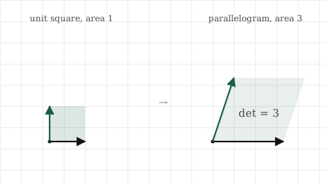
We begin with the unit square, which has an area of exactly one. When we apply a transformation, the square becomes a parallelogram. The two sides of this new shape are the landing spots of the basis vectors. These are the two columns of the matrix. The determinant is simply the area of that resulting parallelogram compared directly against the original square.
If the parallelogram has an area of three, the determinant is three. This means the transformation triples all areas. It does not just triple this one specific square. It triples every area in the entire plane because a linear transformation treats the space uniformly. A region with an area of five would expand to an area of fifteen under this exact same matrix. The determinant is a single scaling factor that applies everywhere simultaneously. If the parallelogram has an area of one half, the determinant is one half. The transformation simply shrinks every area to half its original size.
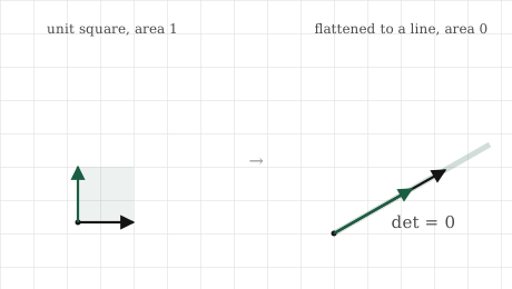
The next scenario carries a massive amount of mathematical meaning. Suppose the transformation sends both basis vectors onto the exact same line. This happens when the two columns of the matrix point in the exact same direction. The unit square is flattened completely onto a single line. Because a flat line has absolutely no physical area, the resulting area is zero. This means the determinant is exactly zero. A zero determinant is the distinct signature of a transformation that completely collapses space. It flattens the plane onto a line or a single point, permanently destroying a dimension in the process.
This connects directly to the concepts from the previous chapter. A transformation with columns pointing the same way has dependent columns. This means it is a rank-deficient transformation. A zero determinant and a deficient rank describe the exact same event from two different perspectives. The columns fail to be independent. The space they reach collapses into a lower dimension. Finally, the physical area of that collapsed image becomes zero. The determinant provides a single number that instantly detects the same collapse we previously learned to count using rank.
There is one final detail the area calculation carries. It includes a mathematical sign. If a transformation flips the plane over like turning a page, it reverses the physical orientation of the space. We record this reflection by making the determinant negative. A determinant of \(-2\) means the physical areas are doubled, but the space itself is flipped backward. The numerical size of the determinant represents the area scaling factor. The positive or negative sign tells us whether the transformation preserved the original orientation or turned it inside out. The magnitude is our main focus right now, but the sign is a deliberate and genuine part of the final number.
For a simple two-by-two matrix, the area of the parallelogram follows a very short formula. This is the only piece of determinant arithmetic you truly need to memorize. If we have a matrix:
\[A = \begin{bmatrix} a & b \\ c & d \end{bmatrix},\]
then its determinant is calculated as:
\[\det(A) = ad - bc.\]
The columns are \([a, c]\) and \([b, d]\), which represent the two physical sides of the parallelogram. The calculation \(ad - bc\) yields the exact area that the shape encloses while also capturing the orientation sign. We will not walk through the long geometric proof of why this specific combination calculates the area. It stems from finding the base and height of the parallelogram using raw coordinates. The full details are available in the appendix. The most important skill is learning how to read the result and trusting what it actually measures.
We can test this formula against the scenarios we already visualized. The identity matrix leaves everything completely unchanged. Its values are \(a = 1\), \(b = 0\), \(c = 0\), and \(d = 1\). The formula gives \(\det(A) = 1\cdot1 - 0\cdot0 = 1\). The area is mathematically unchanged. This perfectly matches a transformation that does absolutely nothing to the space.
Now consider a matrix that doubles both main axes. We set \(a = 2\) and \(d = 2\), leaving the others at zero. The formula gives \(\det(A) = 4\). Doubling two separate dimensions quadruples the total area, which perfectly matches doubling the physical sides of a square.
Finally, we can test a collapse. We use the columns \([1, 2]\) and \([2, 4]\), where the second is just twice the first. The formula gives \(\det(A) = 1\cdot4 - 2\cdot2 = 0\). This zero clearly signals the square was flattened entirely onto a line.
In three dimensions, the determinant measures physical volume rather than a flat area. It measures the volume of the slanted shape that a standard unit cube becomes. The calculation formula grows much longer, but the underlying meaning remains completely identical. It is simply the factor by which the transformation scales volume. It still returns zero when the transformation collapses the cube perfectly flat. In higher dimensions, the determinant is always the single numerical factor for how a transformation scales the physical content of the space. A result of zero always means a structural collapse. The arithmetic formulas become highly elaborate, but the core concept never changes.
The determinant requires just one function call in Python. We will confirm the geometry manually first. We want to prove the two-by-two formula accurately calculates the area scaling, and that zero genuinely marks a structural collapse.
Start with the manual formula on a matrix that doubles areas:
import numpy as np
A = np.array([[2.0, 0.0],
[0.0, 2.0]])
a, b = A[0, 0], A[0, 1]
c, d = A[1, 0], A[1, 1]
print(a * d - b * c)4.0The output is exactly four, matching our earlier logic. Doubling both axes stretches the overall area by a factor of four. NumPy provides this directly as a built-in function:
print(np.linalg.det(A))4.0The function outputs the same result of four. Now we can observe a mathematical collapse. We will define a matrix where the second column is twice the first. This guarantees the columns are dependent:
collapse = np.array([[1.0, 2.0],
                     [2.0, 4.0]])
print(np.linalg.det(collapse))0.0The result is zero, ignoring the tiny floating-point decimals that computer processors occasionally leave behind. The determinant successfully detected that this transformation flattens the entire plane onto a single line. This observation aligns perfectly with what the rank measurement says about the exact same matrix:
print(np.linalg.matrix_rank(collapse))1The rank is precisely one. There is only one independent direction, proving the collapse using a different counting method. The zero determinant and the deficient rank represent the exact same geometric fact reported by two different tools.
Finally, we can test the mathematical sign to see an orientation flip. We will create a matrix that completely swaps the two axes. It sends \([1,0]\) to \([0,1]\) and \([0,1]\) to \([1,0]\). This physically reflects the plane:
flip = np.array([[0.0, 1.0],
                 [1.0, 0.0]])
print(np.linalg.det(flip))-1.0The output is negative one. The numerical magnitude of one proves the areas are preserved and nothing was stretched. The negative sign proves the plane was physically turned over in the process. The determinant successfully reported both the size scaling and the geometric flip in a single number.
The determinant serves primarily as a mathematical alarm bell in machine learning. A zero determinant proves a transformation has completely collapsed the space. This collapse is the exact condition that causes many complex operations to fail. The most common failure happens when trying to invert a matrix to undo a transformation. If a transformation flattened a plane onto a line, it is physically impossible to reverse the process. Every point on that new line originated from many different starting points in the original plane. An undo operation cannot know which specific starting point to choose. Vital information was permanently destroyed during the collapse, and no inverse function can ever recover it. A zero determinant is the exact signal that a transformation cannot be reversed. We will rely on this heavily in the next chapter when checking if a system of equations has a unique answer.
In practical programming, the danger is rarely a determinant of exactly zero. The real danger is a determinant sitting very close to zero. This signals a transformation that nearly collapsed the space, squashing it almost completely flat. Undoing this specific transformation is theoretically possible, but it is highly dangerous in practice. Tiny decimal errors in the input data will be magnified enormously because the near-collapse must be violently forced back open. A matrix with a near-zero determinant is called an ill-conditioned matrix. This is a very common source of numerical failure in machine learning. Models that attempt to invert an ill-conditioned matrix will generate wildly unstable results. Monitoring the determinant helps developers know if a computation can actually be trusted.
The determinant also appears in advanced models that transform probability distributions. Many modern generative models take a very simple probability distribution and push it through a series of transformations to create a highly complex one. When you stretch or compress a mathematical space, you stretch or compress the probability density living inside it. The factor by which that density changes is exactly equal to the determinant of the transformation. These advanced models must calculate determinants constantly to track how the probability mass redistributes as it moves through each layer. The basic area-scaling concept from our simple unit square acts as the strict accounting system that keeps the model accurate.
The determinant measures the physical transformation, not the raw numbers. The simple formula of \(ad - bc\) makes the determinant look like a basic arithmetic combination of the matrix entries. It is actually the geometric area-scaling factor of the transformation. The arithmetic is simply the easiest way we compute that factor. Two matrices with completely different numbers can easily share the exact same determinant. They simply scale the overall area by the same amount while moving the space in entirely different ways. You must view the determinant as a measurement of physical content, not just a sum of products.
A zero determinant does not push everything to the origin. A collapse means the plane is flattened onto a line, or a three-dimensional space is crushed flat onto a plane. It does not mean every data point is sent to the zero coordinate. Many points easily survive a structural collapse. They are just squashed together into a lower dimension. The final image is a solid line full of overlapping points, not one single dot. A zero determinant strictly means zero area, not zero output.
Do not test for exact zero in your code. The collapse example we ran earlier did not print a perfectly clean zero. It printed a tiny speck of floating-point arithmetic dust, looking something like \(-2 \times 10^{-16}\). We have discussed this hardware approximation issue before. It means a strict programming test like det == 0 will almost always return False even when checking a genuinely collapsed matrix. The processor calculation is always slightly off. The safe approach is to check if the determinant is incredibly close to zero relative to the overall scale of the matrix. Relying on an exact zero test for a computed determinant is a guaranteed way to introduce quiet bugs.
A large determinant does not imply an important matrix. The determinant strictly measures area scaling. A matrix can hold massive internal numbers and still return a zero determinant if it completely collapses the space. Alternatively, a matrix can have a very small determinant while stretching one direction massively and squashing another. The determinant only reports the final net effect on the total area. It does not measure the overall size or significance of the data. If we want to know how much a transformation stretches specific individual directions, we must use singular values, which we cover in a later chapter. The determinant only summarizes the combined area effect.
Try to answer these questions before looking at the answers.
1. A transformation has determinant \(5\). You apply it to a shape of area \(2\). What is the area of the result?
2. A two-by-two matrix has columns \([3, 1]\) and \([6, 2]\). Without computing \(ad - bc\), what do you expect its determinant to be, and why?
3. A transformation has determinant \(-1\). What does it do to areas, and what does the sign tell you?
4. Matrix \(A\) has determinant \(3\) and matrix \(B\) has determinant \(4\). You apply \(B\) first, then \(A\). By what factor does the combined transformation scale area?
5. You are about to invert a matrix as part of fitting a model, and you notice its determinant is \(0.0000001\), very close to zero. Should you be comfortable? What does this tell you about the computation ahead?
1. The final area is ten. The determinant is the multiplier for every area in the space. An area of two becomes \(2 \times 5 = 10\). The determinant applies uniformly to every region, regardless of its shape or size.
2. The determinant is zero. The second column \([6, 2]\) is exactly twice the first column \([3, 1]\). Because the two columns point in the exact same direction, they are dependent. The parallelogram they form is completely flattened onto a line, leaving no area. A collapse always produces a zero determinant, and we can spot this directly from the columns without needing the formula. The basic arithmetic also confirms this, since \(3\cdot2 - 6\cdot1 = 0\).
3. It preserves the exact physical areas because the numerical magnitude of the determinant is strictly one. It also physically flips the plane over because the sign is negative. Nothing is stretched or shrunk in the process. The shape keeps its original size, but its orientation is entirely reversed, similar to a reflection in a mirror. The magnitude dictates the size, and the sign dictates the handedness.
4. The final factor is twelve. Composing transformations simply multiplies their individual area-scaling factors together. The first matrix scales the area by four. The second matrix scales that newly adjusted area by three. This provides a total factor of \(4 \times 3 = 12\). The determinants of composed transformations simply multiply, which aligns perfectly with scaling an area and then scaling it again.
5. You should be highly cautious. A determinant sitting that close to zero means the matrix nearly collapses the entire space. Inverting a near-collapse is numerically treacherous. Tiny errors in your original data will be magnified dramatically in the final result. The model’s output will likely become unstable and completely untrustworthy. This matrix is ill-conditioned. It is technically possible to proceed, but the near-zero determinant is a massive warning that the math ahead is fragile and the final answer may be wrong.