import numpy as np

A = np.array([[2.0, 3.0],
              [1.0, -1.0]])
b = np.array([12.0, 1.0])9 Systems of Equations, Geometrically
The itch
Somewhere in school, most of us encountered equations like \(2x + 3y = 12\) and \(x - y = 1\). We had two equations and two unknowns, and we were taught to grind them into a solution using elimination or substitution. It worked, but it felt like arithmetic in the dark. Nothing about the procedure explained what we were really doing or why an answer actually existed. We have spent six chapters building the machinery to see this clearly. Now, the whole subject snaps into a single visual picture.
We can reframe the problem by stacking those equations into a matrix acting on a vector of unknowns. The two previous equations look exactly like this:
\[\begin{bmatrix} 2 & 3 \\ 1 & -1 \end{bmatrix} \begin{bmatrix} x \\ y \end{bmatrix} = \begin{bmatrix} 12 \\ 1 \end{bmatrix}\]
This is simply \(A\mathbf{x} = \mathbf{b}\). You should read this as a transformation. The matrix \(A\) is the transformation, \(\mathbf{x}\) is some unknown starting vector, and \(\mathbf{b}\) is the final destination where \(\mathbf{x}\) lands after \(A\) acts on it. We know the transformation and we know the final destination. The question asks where we started. We need to know which specific vector \(\mathbf{x}\) the transformation \(A\) sends to \(\mathbf{b}\).
This is what solving a system of equations actually means. It is not about grinding through elimination. It is about running a transformation backward to find where something began based on where it landed. Once we view it this way, everything we already know about transformations tells us immediately if the system has one answer, no answer, or infinitely many. The dark arithmetic transforms into a logical geometric question about undoing a known motion.
The picture
Think of solving \(A\mathbf{x} = \mathbf{b}\) as a geometric search. The transformation \(A\) takes every vector to a new location. We are told that some particular vector \(\mathbf{x}\) was taken to \(\mathbf{b}\), and we want that \(\mathbf{x}\) back. If we could run \(A\) in reverse, we would apply that reverse motion to \(\mathbf{b}\) and arrive at \(\mathbf{x}\) directly. Solving the system simply asks if \(A\) can run in reverse, and then executes that reverse motion.
For a well-behaved transformation that does not collapse space, running it in reverse always works perfectly. Every output comes from exactly one input because a non-collapsing transformation never sends two different vectors to the exact same place. This means there is a single vector that lands on \(\mathbf{b}\), guaranteeing the system has exactly one solution. Geometrically, \(A\) stretches, rotates, and shears the space without ever flattening it. This means we can perfectly undo those moves and walk \(\mathbf{b}\) back to its unique origin.
We must also consider the case where the system breaks, which is the geometric collapse from the last two chapters. Suppose \(A\) flattens the entire plane onto a single line. This is a rank-deficient transformation with a zero determinant. In this scenario, many different input vectors all get squashed onto the exact same output location. Running the transformation backward is no longer a well-defined process. Given a point on that line, we cannot say which of the many vectors that landed there was our original \(\mathbf{x}\). The destination \(\mathbf{b}\) now decides between two possible fates.
If \(\mathbf{b}\) does not lie on the specific line that \(A\) squashes everything onto, then absolutely nothing maps to \(\mathbf{b}\). No input ever lands there, meaning there is no mathematical solution. The equations are asking for a vector that cannot possibly exist.
If \(\mathbf{b}\) does sit precisely on that line, the exact opposite problem appears. A whole infinite family of vectors maps to that exact coordinate. The system has infinitely many solutions forming an entire line, and no single answer can be separated from the rest. A geometric collapse turns one clean answer into either zero answers or endlessly many. The final outcome depends entirely on whether the target survived the collapse.
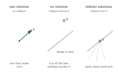
The three classic possibilities of a linear system are one solution, no solution, and infinitely many solutions. The old elimination method produced these as mysterious mathematical special cases. However, they are not mysterious at all. They simply describe whether the transformation collapses space, and if so, whether the target sits inside that collapsed image. Everything can be read directly from the geometry.
The math, built up
Running a transformation backward has a specific name and notation. When \(A\) does not collapse the space, there is a reliable transformation that undoes it. This is called the inverse of \(A\), and it is written as \(A^{-1}\). It is the transformation that takes every landing spot directly back to where it came from, meaning applying \(A\) and then \(A^{-1}\) returns every vector perfectly unchanged. Using this, the solution to the system becomes immediate:
\[A\mathbf{x} = \mathbf{b} \quad\Longrightarrow\quad \mathbf{x} = A^{-1}\mathbf{b}.\]
You simply apply the undoing transformation to the destination, and you arrive at the unique starting point. This is the entire solution compressed into one clear line. To solve the system, you just run the transformation backward on \(\mathbf{b}\).
The inverse exists exactly when the transformation does not collapse the space. We now have several equivalent ways to state this fact. The inverse exists when the determinant is not zero. It exists when the columns are fully independent. It exists when the matrix has full rank. A matrix containing an inverse is called invertible. Invertible, non-zero determinant, full rank, and independent columns are simply four different names for the exact same property. They all confirm the transformation preserves space instead of flattening it, allowing the process to be undone.
When that property fails, the inverse does not exist. There is no single transformation that undoes a collapse because the collapse permanently destroyed the information needed to trace the path backward. This explains why a system with a collapsing matrix has no clean solution. The system might still have the infinitely many solutions we discussed earlier, but you cannot reach them by inverting the matrix because there is nothing to physically invert.
We will not write out the manual formula for computing an inverse. For a simple two-by-two case, it is a rearrangement of the entries divided by the overall determinant. This reveals the core problem instantly. The determinant sits in the denominator of the fraction. A zero determinant means dividing by zero, which causes the math to blow up exactly when the transformation collapses. In practice, the inverse is always computed by a machine. Often, it is not formally computed at all because there are cheaper ways to solve the system without building the entire undoing transformation. The geometric meaning is what truly matters. Solving is undoing, and undoing is possible exactly when the transformation preserves the space.
Build it yourself
We will now solve a system by running the transformation backward in Python. Then we will watch what happens when the transformation collapses.
Here is the system from the start of the chapter, defined as a matrix and a target:
The determinant is not zero, so \(A\) does not collapse space and can safely run backward. We can form the formal inverse and apply it to \(\mathbf{b}\), exactly as our mathematical formula states:
A_inv = np.linalg.inv(A)
x = A_inv @ b
print(x)
[3. 2.]The solution is \([3, 2]\). The transformation \(A\) successfully sends the vector \([3, 2]\) to the coordinates \([12, 1]\). We recovered the start by completely undoing the motion. We can verify this by going forward again, applying \(A\) to our answer to ensure it lands exactly on \(\mathbf{b}\):
print(A @ x)[12. 1.]The output returns back to \([12, 1]\), which is the destination we were given. The undoing process was entirely correct.
In real programming, you rarely build the formal inverse. You ask the solver for \(\mathbf{x}\) directly, which is mathematically faster and much more stable:
x = np.linalg.solve(A, b)
print(x)
[3. 2.]The system outputs the same \([3, 2]\). The np.linalg.solve function runs the transformation backward without constructing the massive inverse transformation in memory. This is the correct method to reach for in practical work.
We can now test a collapsing system. The two rows describe the exact same direction, causing the matrix to flatten the plane completely:
A_bad = np.array([[1.0, 2.0],
                  [2.0, 4.0]])
b_bad = np.array([3.0, 99.0])

print(np.linalg.det(A_bad))0.0The system calculates a determinant of zero, which is the signature of a structural collapse. Asking the computer to undo this process fails because there is absolutely nothing to undo:
try:
    np.linalg.inv(A_bad)
except np.linalg.LinAlgError as e:
    print("no inverse:", e)
no inverse: Singular matrixThe library refuses to proceed, reporting a singular matrix. This is the formal term for a collapsing, non-invertible transformation. The geometry predicted this outcome exactly. A flattened transformation cannot run backward, so the system it defines has no clean geometric solution to hand back.
Where it lives in ML
Solving \(A\mathbf{x} = \mathbf{b}\) is a central pillar of machine learning. A massive amount of what classical models do ultimately comes down to setting up a system of linear equations and solving it. The most direct example is linear regression. Fitting a straight relationship to data creates a system in this exact format. The best-fit answer is found by running a transformation backward to recover the specific weights that produced the data.
Real data makes this story much richer. When we fit a model, we usually have far more equations than unknowns. We might have thousands of demands placed on just a few numbers. A system like this almost never has a perfect exact solution. The equations contradict each other slightly because real-world data carries noise. No single choice of weights can satisfy all the equations simultaneously. In the strict mathematical sense, there is no exact solution because the target \(\mathbf{b}\) does not sit perfectly inside the reachable image.
Rather than giving up, we simply change the question. Instead of demanding a vector that lands perfectly on \(\mathbf{b}\), we look for the one that lands as close to \(\mathbf{b}\) as possible. We measure this distance using the straight-line L2 norm we built earlier. This is called the least-squares solution. It is exactly what fitting a model actually computes. We abandon the impossible exact answer and accept the nearest reachable one. This approach relies on the concept of the reachable image from this chapter combined with the measurement logic from the norms chapter.
The geometric collapse matters here as a severe practical warning. When the features of a dataset are highly redundant, the system is nearly collapsing. The transformation we need to invert becomes singular or ill-conditioned. The model cannot find a unique answer, or it finds a wildly unstable one. This happens for the exact geometric reason we laid out. There is no clean way to run a structural collapse backward. Recognizing a rank-deficient system and repairing it before solving is a mandatory part of making a model work reliably.
Common misunderstandings
Solving a system is undoing a transformation, not just manipulating rows. The standard elimination procedures taught in school are simply one way to compute the answer. They do not explain what solving actually means. We are physically running a transformation backward to recover an original input from its output. Holding onto this geometric meaning allows you to predict if a solution exists before doing any computation. The row manipulations are just a means to an end, while the undoing is the true mathematical meaning.
No solution and infinitely many solutions are opposite situations. It is very easy to lump these two cases together and assume the system simply broke. They are actually precise opposites. Having no solution means the target lies completely outside the reachable image. Having infinitely many solutions means the target lies inside a collapsed image that many different inputs share. Both issues stem from a collapsing transformation, but the final result depends entirely on where the target sits.
The existence of an inverse is a property of the matrix, not the target. Whether the inverse exists depends entirely on the matrix and whether the transformation collapses the space. It does not depend on the target \(\mathbf{b}\) at all. When a matrix is invertible, every possible target has exactly one unique solution. The target only decides the outcome when the transformation has already collapsed. You must keep the physical properties of the matrix completely separate from the properties of the target destination.
In practice, you rarely want to compute the actual inverse. Beginners often try to compute the formal inverse and then multiply because the standard formula heavily suggests it. Building the entire undoing transformation is significantly more work and numerically unstable. This is exactly why standard programming libraries offer a solver function that never explicitly forms the inverse. You should reserve the formal inverse for situations where you genuinely need the entire undoing transformation, rather than just the answer to one specific system.
Check your intuition
Try to answer these questions before opening the answers below.
1. A transformation \(A\) does not collapse space. How many solutions does \(A\mathbf{x} = \mathbf{b}\) have, and does the answer depend on which \(\mathbf{b}\) you pick?
2. You are told \(\det(A) = 0\). What are the possible numbers of solutions to \(A\mathbf{x} = \mathbf{b}\), and what decides between them?
3. A system \(A\mathbf{x} = \mathbf{b}\) has infinitely many solutions. What does this tell you about the transformation \(A\), and about where \(\mathbf{b}\) sits?
4. You try to solve a system and the library reports the matrix is “singular.” In the language of this book, what has it found?
5. A dataset has one thousand data points and three weights to fit, giving a system with a thousand equations and three unknowns. Do you expect an exact solution? If not, what do we look for instead?
TipAnswers
1. There is exactly one solution, and this holds absolutely true for every possible \(\mathbf{b}\). A non-collapsing transformation is perfectly invertible, so it runs backward uniquely. Every target came from exactly one starting location. Because invertibility is a property of \(A\) alone, the strict guarantee of a single solution applies no matter which target you choose.
2. A zero determinant proves that \(A\) collapses space. The system has either no solution or infinitely many solutions. Which of the two occurs is decided completely by the target \(\mathbf{b}\). If \(\mathbf{b}\) lies within the collapsed image, there are infinitely many solutions. If \(\mathbf{b}\) lies outside the collapsed image, there are absolutely none. The zero determinant removes the possibility of a unique answer, and the target dictates the final result.
3. The transformation \(A\) collapses the space. It is mathematically singular, rank-deficient, and possesses a zero determinant. Furthermore, \(\mathbf{b}\) sits directly inside the collapsed image, which is the line or plane that \(A\) squashes everything onto. Because infinitely many inputs get mapped onto that exact image, a whole family of vectors lands precisely on \(\mathbf{b}\). A reachable target combined with a collapsing transformation produces the infinite family of solutions.
4. The library has found that the matrix collapses space. The transformation is non-invertible, its determinant is exactly zero, its columns are completely dependent, and its rank is formally deficient. The term singular is the formal mathematical name for all of these problems occurring at once. The computer library is telling you there is no clean geometric answer to provide.
5. No exact solution should be expected here. A thousand distinct equations pressing on three unknowns will almost always contradict one another because real data contains noise. No three individual weights can perfectly satisfy every equation simultaneously. The mathematical target does not lie precisely in the reachable image. Instead of an impossible exact answer, we actively search for the least-squares solution. We want the weights that land as close to the target as physically possible in a straight-line distance.