import numpy as np

A = np.array([[3.0, 0.0],
              [0.0, 1.0]])

values, vectors = np.linalg.eig(A)
print(values)
print(vectors)
[3.+0.j 1.+0.j]
[[1.+0.j 0.+0.j]
[0.+0.j 1.+0.j]]When a transformation acts on a flat plane, it treats almost every single vector differently. It actively turns them. An arrow pointing in one specific direction gets forcefully swung to point somewhere else. Its length changes, but more importantly, its direction changes. If you watch a shearing motion or a rotation act on a fan of arrows, they all pivot, and each one ends up aimed at a new target. A transformation generally does not preserve direction; turning things is its primary job.
However, not every arrow turns. For most transformations, there are a few highly specific directions that survive the process completely unturned. A vector pointing exactly along one of these special directions gets stretched or squashed, making it physically longer or shorter. Crucially, it keeps pointing in the exact same direction it did originally. The transformation simply moved the arrow along its own line without ever knocking it off balance. These survivor directions are quite rare, usually limited to just one or two in a standard plane, while everything else pivots dramatically around them.
Those special survivor directions represent the deep mechanical structure of the transformation. They are the core axes the transformation is mathematically built around. They are the specific directions the transformation treats in the simplest possible way, using pure stretching with absolutely no turning. If we can isolate them, a highly complicated transformation resolves into something much easier to understand. Along these specific directions, the matrix merely scales the data. The entire complex behavior of the matrix can be read by looking at what it does to these core lines. This chapter focuses on finding those specific directions and measuring the exact amounts they get stretched. These measurements are among the most useful things a matrix can ever tell us.
Imagine a transformation and watch what it does to arrows pointing in every possible direction. Nearly all of them get forcefully turned. The original arrow and its newly transformed version point in different ways because the transformation swung the arrow off its original path. If you picture the starting arrow and its final image drawn from the origin, they almost always form a distinct angle. This angle is clear geometric evidence that the direction was not preserved.
Now we must hunt for the rare exceptions. Is there a specific direction where the original arrow and its transformed image still lie perfectly along the exact same line? We are looking for a place where the transformation, regardless of whatever else it accomplished, did not swing the arrow off course. It only slid the arrow along its own line, perhaps making it longer, shorter, or facing backward, but never turning it. For most standard transformations, these specific directions do exist, and they are mathematically special enough to require formal names. A direction that perfectly survives a transformation unturned is called an eigenvector of that transformation. The numerical factor by which that specific arrow gets stretched is called its eigenvalue.
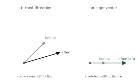
A practical example makes these two concepts concrete. Consider a transformation that stretches everything horizontally by a factor of three but leaves the vertical direction completely untouched. A vector pointing straight along the horizontal axis gets tripled in physical length, but it stays perfectly horizontal. Therefore, it is an eigenvector with an eigenvalue of exactly three. A vector pointing straight up is left completely alone and unmoved. It is also an eigenvector with an eigenvalue of exactly one because it is stretched by a factor of one, meaning not at all. However, a vector pointing diagonally gets pulled flatter because its horizontal part triples while its vertical part stays put. It ends up aimed differently than it began. The diagonal direction was actively turned, so it is not an eigenvector. The two main axes survive the process perfectly, but the diagonal does not.
Eigenvalues carry a mathematical sign and a physical size, and both convey a clear meaning. An eigenvalue larger than one proves the eigenvector is being stretched outward. An eigenvalue between zero and one proves the vector is being squashed inward toward the origin. An eigenvalue of exactly one means the vector is left perfectly unchanged. A negative eigenvalue means the arrow is flipped to point completely backward along its own line. This still counts as unturned because it stays trapped on the exact same line through the origin, just facing the opposite way. Finally, an eigenvalue of exactly zero means the eigenvector is squashed entirely to nothing, collapsing perfectly onto the origin. This represents the specific direction a collapsing transformation actively destroys.
Not every single transformation possesses these survivor directions in the flat plane. A pure rotation, which turns every single arrow by the exact same angle, naturally turns all of them. Therefore, it has no real eigenvectors at all because no direction survives a quarter-turn unturned. This is not a flaw in the underlying mathematics. It is the math correctly reporting that a true rotation preserves absolutely no direction. When survivor directions do exist, they expose the true skeleton of the transformation.
This visual picture translates smoothly into one compact mathematical equation. An eigenvector is a specific vector \(\mathbf{v}\) that the transformation \(A\) sends perfectly to a scaled copy of itself. It is stretched by the eigenvalue \(\lambda\) but not turned:
\[ A\mathbf{v} = \lambda \mathbf{v}. \]
You should read each side of the equation through our geometric picture. The left side, \(A\mathbf{v}\), represents the full transformation acting heavily on the vector, sending it wherever it naturally goes. The right side, \(\lambda\mathbf{v}\), is that exact same vector merely scaled, remaining perfectly on its own line. The equation explicitly states these two outcomes are equal. Applying the entire complex transformation to \(\mathbf{v}\) accomplishes nothing more than stretching it by \(\lambda\). That is the entire formal definition. It is simply the survivor-direction concept written in algebra.
There is a subtle point the equation makes very clear. If \(\mathbf{v}\) is a valid eigenvector, then any scaled copy of it is also a valid eigenvector. Stretching a survivor direction just produces another arrow trapped on the exact same line, equally unturned. This means eigenvectors exist as entire continuous lines, not just single isolated arrows. The geometric direction is what truly matters, although we usually pick one representative arrow along that line, often scaled to a clean length of one. The eigenvalue, in contrast, is a single fixed number. It tells us exactly how much that specific direction gets stretched, and it remains identical regardless of which representative arrow we chose.
Finding the eigenvectors requires finding the specific \(\mathbf{v}\) and \(\lambda\) that satisfy the equation. The logical route to finding them runs straight through the lessons of the last two chapters. We can rearrange the equation so one side equals zero. We want \(A\mathbf{v} - \lambda\mathbf{v} = \mathbf{0}\). We can treat \(\lambda\mathbf{v}\) as a transformation that simply scales \(\mathbf{v}\) by \(\lambda\). This turns the equation into \((A - \lambda I)\mathbf{v} = \mathbf{0}\), where \(I\) is the standard identity matrix. This new equation states that the specific transformation \(A - \lambda I\) sends a non-zero vector \(\mathbf{v}\) perfectly to the origin. However, any transformation that sends a non-zero vector completely to zero is a collapsing transformation. We know the exact mathematical signature for that event: its determinant must equal zero. Therefore, the true eigenvalues are precisely the specific numbers \(\lambda\) that satisfy:
\[ \det(A - \lambda I) = 0. \]
This equation forms the necessary bridge from our visual picture to a raw computation. Every specific \(\lambda\) that forces \(A - \lambda I\) to collapse is a valid eigenvalue. For each of those valid \(\lambda\) values, the specific directions that get sent perfectly to zero become its eigenvectors. We will not turn this into a manual hand procedure by solving the resulting equation for \(\lambda\) and substituting values backward. For anything beyond the smallest textbook matrices, this process is always handled by a computer. The critical takeaway is that eigenvalues are the stretch factors, eigenvectors are the survivor directions, and the entire search reduces to asking when a related transformation collapses. This links eigenvectors directly back to the determinant and rank concepts we already built.
Finding eigenvectors completely by hand is highly laborious. Fortunately, NumPy handles it perfectly in one function call, allowing us to verify the survivor-direction picture directly using code.
We will start with the horizontal stretch from our earlier visual example. It triples the first axis and leaves the second axis alone:
import numpy as np
A = np.array([[3.0, 0.0],
[0.0, 1.0]])
values, vectors = np.linalg.eig(A)
print(values)
print(vectors)[3.+0.j 1.+0.j]
[[1.+0.j 0.+0.j]
[0.+0.j 1.+0.j]]The system returns eigenvalues of three and one. These are the exact two stretch factors we reasoned out logically. The eigenvectors are returned neatly as the vertical columns of the second array. They are the pure horizontal and vertical directions, each presented as a unit-length arrow. The transformation’s survivor directions are exactly the two main axes, perfectly matching our visual promise.
Now we can confirm the defining mathematical property directly. Applying \(A\) to an eigenvector should equal simply scaling that specific eigenvector by its exact eigenvalue. We will take the first eigenvector and its corresponding eigenvalue and check both sides of \(A\mathbf{v} = \lambda\mathbf{v}\):
v = vectors[:, 0]           # extract the first eigenvector
lam = values[0]             # extract its matching eigenvalue

print(A @ v)                # the transformation acting heavily on v
print(lam * v)              # v merely scaled by the eigenvalue
[3.+0.j 0.+0.j]
[3.+0.j 0.+0.j]The two output lines print the exact same vector. Applying the entire complex transformation to this specific direction achieved nothing more than a simple scaling. This is precisely what makes it an eigenvector. The arrow was not turned; it was only stretched.
We can watch a turned direction fail this exact same test. A diagonal vector is not a true eigenvector of this transformation. Therefore, applying \(A\) to it should not result in a mere scaling:
d = np.array([1.0, 1.0])    # define a diagonal direction
print(A @ d)                # becomes [3, 1]
[3. 1.]The diagonal vector \([1, 1]\) becomes \([3, 1]\). It clearly does not point the same way as \([1, 1]\) because the direction was turned and pulled flatter. No single numerical number can cleanly scale \([1, 1]\) directly into \([3, 1]\). This failure is precisely what it means for a direction to not be an eigenvector.
Finally, the rotation matrix with no survivors behaves exactly as the visual picture warned us. A quarter-turn rotates every single direction, so it should not have any real eigenvectors at all:
R = np.array([[0.0, -1.0],
              [1.0,  0.0]])
print(np.linalg.eig(R).eigenvalues)
[0.+1.j 0.-1.j]The system returns complex numbers rather than real ones. This is simply the arithmetic’s way of reporting that absolutely no real direction survives the rotation unturned. When a transformation preserves no direction, the real survivor directions simply do not exist to be found.
Eigenvectors matter deeply in machine learning because they locate the directions that actually matter inside the data. The most prominent example is a technique we have referenced for several chapters: principal component analysis, or PCA. The sole job of PCA is to look at a massive cloud of data and locate the specific directions along which the data varies the most. It finds the core axes the data is truly organized around so we can keep those few vital directions and discard the rest. Those specific directions of greatest variation are simply eigenvectors of a specialized matrix built from the raw data. Their corresponding eigenvalues tell us exactly how much variation each direction carries. PCA is, at its core, just an eigenvector computation. Dimensionality reduction simply means keeping the eigenvectors attached to the largest eigenvalues and throwing away the small ones.
This process works because the survivor-direction idea naturally applies to raw data. A dataset scattered through a high-dimensional space usually has a few core directions along which it stretches out significantly, and many directions along which it barely moves. The high-eigenvalue directions are where the valuable information lives. The low-eigenvalue directions are practically flat, carrying almost nothing useful. Reducing the data down to its top few eigenvectors preserves almost all of the internal structure while collapsing the physical description from thousands of complex numbers down to a manageable handful. This fulfills the low-rank hope from the independence chapter, making it fully actionable. The eigenvalues explicitly tell us which directions are mathematically worth keeping.
Eigenvalues also diagnose the complex behavior of repeated transformations. These appear constantly in machine learning whenever a process is applied over and over again. When a transformation is applied sequentially many times, its eigenvalues dictate what happens in the long run. Any directions with an eigenvalue larger than one will physically grow with each application. If the process runs long enough, they will explode mathematically. Any directions with an eigenvalue smaller than one will physically shrink away to nothing. This math perfectly explains a famous difficulty in training deep and recurrent neural networks. Signals passed through many successive layers either blow up violently or vanish completely depending on whether the relevant eigenvalues sit above or below one. The exploding and vanishing gradients that heavily plague deep learning are fundamentally a story about the eigenvalues of a repeated geometric transformation.
There is another appearance that is highly relevant to the systems discussed in this book. The numerical stability of many iterative training methods is dictated by eigenvalues. The way a training process either settles cleanly toward a final answer or spirals out of control is read directly through the eigenvalues of the transformation each step applies. Whether a complex method successfully converges is often precisely a question of whether certain key eigenvalues rest safely inside a specific range. The survivor directions and their stretch factors often dictate whether the most critical processes in the entire field will function at all.
An eigenvector is an entire direction, not a single arrow. Because any valid scaling of an eigenvector remains a valid eigenvector trapped on the same unturned line, it makes no sense to refer to the eigenvector as one specific physical arrow. The true eigenvector is the entire continuous line running through the origin. It is the geometric direction that survives. Computer tools will return a single representative arrow, usually scaled to a clean length of one. However, that particular arrow is just an arbitrary choice of representative, not the fundamental eigenvector itself. The only fixed and meaningful properties are the direction and its associated eigenvalue.
Not every transformation has real eigenvectors. It is highly tempting to assume survivor directions always exist somewhere in the space. However, a pure rotation turns every single direction and preserves none, meaning it has absolutely no real eigenvectors. The computer computation honestly reports this fact by returning complex numbers instead of real ones. This is not a failure of the algorithm. It is the correct mathematical answer that no real direction comes through unturned. When you expect clean eigenvectors and receive complex values, the transformation is performing a rotational motion. It is mixing directions together rather than simply stretching along fixed axes.
A large eigenvalue does not automatically mean an important eigenvector. For the specialized symmetric matrices that arise in PCA, the eigenvalues do genuinely rank the directions by their true importance, making it safe to keep the largest ones. However, for a standard general matrix, an eigenvalue only dictates the physical stretch along its direction. A large physical stretch does not always equal structural importance. The clean instruction to keep the biggest eigenvalues belongs strictly to the well-behaved matrices used in dimensionality reduction, not to every random matrix. This limitation is exactly why the next chapter is necessary. It provides a version of this specific idea that works reliably for absolutely every matrix.
Eigenvalues can easily be negative or zero. A very common assumption is that eigenvalues must be positive stretch factors. A negative eigenvalue physically flips its eigenvector to point entirely backward along the same line. This still counts as unturned because it remains trapped on the exact same line running through the origin. A zero eigenvalue squashes its direction entirely to the origin. Its presence proves the transformation collapsed that specific direction. This connects eigenvalues perfectly back to the determinant. A transformation has a zero eigenvalue exactly when it mathematically collapses, which is exactly when its determinant is zero. Sign and zero values are not edge cases to be ignored; they actively carry the flip and the collapse.
Try to answer these questions before opening the answers below.
1. A transformation stretches the vertical axis by four and leaves the horizontal axis unchanged. What are its eigenvectors and eigenvalues?
2. A vector \(\mathbf{v}\) satisfies \(A\mathbf{v} = -2\mathbf{v}\). Is \(\mathbf{v}\) an eigenvector? What does the transformation do to it, geometrically?
3. A transformation has an eigenvalue of zero. What does this tell you about the transformation, in the language of earlier chapters?
4. Why does a pure rotation of the plane have no real eigenvectors? Answer from the picture, not the arithmetic.
5. A process applies the same transformation over and over to a vector. One direction has eigenvalue \(1.5\) and another has eigenvalue \(0.5\). What happens to each component as the process runs many times?
1. The two eigenvectors are exactly the two main axes. The vertical direction has an eigenvalue of exactly four because a vertical arrow is physically stretched fourfold while remaining strictly vertical. The horizontal direction has an eigenvalue of exactly one because a horizontal arrow is left completely unchanged, effectively stretched by a factor of one. These two axes are the true survivor directions. Every other possible direction gets physically turned as its vertical part quadruples and its horizontal part stays fixed.
2. Yes, \(\mathbf{v}\) is a perfectly valid eigenvector with an eigenvalue of exactly \(-2\). The equation mathematically proves the transformation sends \(\mathbf{v}\) to \(-2\mathbf{v}\). This means \(\mathbf{v}\) is scaled by two and flipped to point in the exact opposite direction along the same line. It remains unturned because it stays trapped on its own line through the origin, but it is doubled in length and physically reversed. Negative eigenvalues always represent this flip-and-scale action.
3. The transformation physically collapses the space. An eigenvalue of zero proves that a specific direction is squashed entirely to the origin. This is exactly what a collapsing, rank-deficient transformation does mechanically, and it guarantees the determinant is exactly zero. A zero eigenvalue is simply another face of the structural collapse we previously identified as a zero determinant, a deficient rank, and mathematical singularity. The transformation cannot be cleanly undone because a geometric direction has been permanently destroyed.
4. A rotation actively turns every single arrow by the exact same angle. To be an eigenvector, a direction must remain perfectly on its own line and merely stretch. A rotation by anything other than a complete half-turn swings absolutely every direction off its original line, with zero exceptions. There is no physical arrow that a genuine rotation leaves pointing perfectly along its original path, so there are no real eigenvectors. The transformation preserves no direction, and the absence of eigenvectors reports that physical reality accurately.
5. The specific direction with the \(1.5\) eigenvalue physically grows. Each sequential application multiplies it by \(1.5\), so after many rounds, it becomes mathematically enormous. The direction with the \(0.5\) eigenvalue physically shrinks. Each application cuts it directly in half, causing it to fade rapidly toward zero. If run long enough, the growing direction will dominate completely, and the shrinking one will practically vanish. This is the underlying mechanic of exploding and vanishing behavior in repeated transformations, decided entirely by whether an eigenvalue sits above or below one.