import numpy as np

v = np.array([2.0, 1.0])
w = np.array([1.0, 3.0])

products = v * w
print(products)
print(np.sum(products))
[2. 3.]
5.0Two chapters ago we asked how a machine could tell that two songs are similar. We turned each song into a vector, which we visualized as an arrow in space. We learned to measure how long one arrow is, and we learned to add and scale them. However, we never answered the actual question. Length tells us about one arrow on its own. Adding and scaling let us build new arrows. None of it tells us how alike two arrows are.
We need to look at what similarity means now that songs are arrows. Two similar songs become two arrows pointing in much the same direction. Two songs with nothing in common become two arrows pointing in different directions. This means similarity is about the angle between two arrows. A small angle means the vectors are alike. A wide angle means they are different. If they point opposite ways, they are completely unalike.
This reframes the whole problem into something very concrete. We do not need to understand music. We only need to measure the angle between two arrows using the lists of numbers the machine holds. If we can turn two lists of numbers into a single number that reveals if they point the same way, we have solved the problem. The recommendation, the face unlock, and the search result all rely on this one number.
There is a single operation that produces this value. It takes two vectors and returns one number. That number contains the angle between them, the shadow one casts on the other, and the similarity we have been looking for. It is called the dot product, and everything in this chapter is about this one operation.
We want the angle between two arrows, but an angle is awkward to measure directly from two lists of numbers. We will approach it through a visual that carries the angle inside it. That visual is the shadow one arrow casts on another.
Take two vectors, \(\mathbf{v}\) and \(\mathbf{w}\), drawn from the same starting point. Imagine light coming straight down onto \(\mathbf{w}\) at a right angle. We want to look at the shadow \(\mathbf{v}\) casts along the line of \(\mathbf{w}\). That shadow has a length, and this length quietly tracks the angle.
Watch what the shadow does as we swing \(\mathbf{v}\) around. When \(\mathbf{v}\) points the exact same way as \(\mathbf{w}\), it lies flat along \(\mathbf{w}\) and its shadow is full length. As \(\mathbf{v}\) tilts away, the shadow shortens. When \(\mathbf{v}\) stands at a perfect right angle to \(\mathbf{w}\), it casts no shadow along \(\mathbf{w}\) at all. The shadow shrinks to nothing. If we tilt \(\mathbf{v}\) further past the right angle, it begins to cast a shadow pointing backwards along \(\mathbf{w}\). We read this as a negative length.
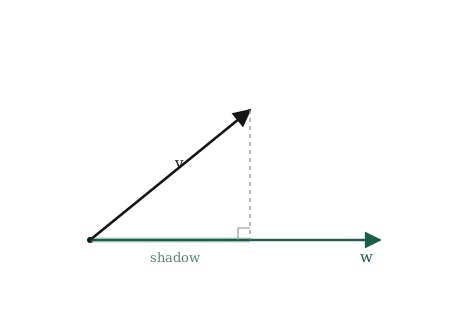
The shadow’s length directly reports on the angle. A full-length shadow means the arrows align. A shrinking shadow means the angle is opening. A zero shadow means a right angle. A negative shadow means they lean opposite ways. We have turned the angle into a length, and length is something we already know how to calculate.
There is one detail to address because it shapes our formula. The shadow depends on two things. It depends on the angle, but it also depends on how long \(\mathbf{v}\) is to begin with. A longer arrow casts a longer shadow at the same angle. When we build the actual operation, it will also include the length of \(\mathbf{w}\). The dot product gives us the angle tangled together with both lengths. Part of the work in this chapter is learning to separate them when we want the angle alone.
We have a visual shadow that represents the angle. We now need to turn it into arithmetic on two lists. Let us build the formula from the simplest possible case.
Start with the two reference vectors from the last chapter, \([1, 0]\) and \([0, 1]\). Ask for the shadow of \([1, 0]\) on \([0, 1]\). One points along the ground, the other straight up at a perfect right angle. The visual shadow is zero. Next, look at the shadow of \([1, 0]\) on itself. The arrow lies flat along its own direction, so the shadow is its full length of one.
Those two facts drive the calculation: - Along the same axis, the shadow is full. - Across a right angle, the shadow is nothing.
Now take two general vectors, \(\mathbf{v} = [v_1, v_2]\) and \(\mathbf{w} = [w_1, w_2]\). We split each into its horizontal and vertical pieces. The \(v_1\) part points purely along the first axis. The \(v_2\) part points purely along the second axis. To ask how much of \(\mathbf{v}\) falls along \(\mathbf{w}\), we add up the contributions piece by piece. Based on our rules, only the matching pieces survive.
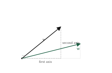
When the first axis meets the first axis, they align and contribute \(v_1 w_1\). The second meets the second, contributing \(v_2 w_2\). When the first axis meets the second axis, they sit at a right angle and contribute nothing. The crossing terms vanish, leaving only a sum of matching products:
\[ \mathbf{v} \cdot \mathbf{w} = v_1 w_1 + v_2 w_2 \]
That is the dot product. You multiply the numbers in matching slots and add the results together. The little dot takes two vectors and returns a single number. That number is the shadow relationship from our picture, written purely in lists the machine can read.
It follows the exact same slot-by-slot pattern as length and addition. It also works no matter how long the lists get. Three hundred numbers means three hundred products summed into one final result:
\[ \mathbf{v} \cdot \mathbf{w} = v_1 w_1 + v_2 w_2 + \cdots + v_n w_n \]
We must clarify one vital point holding this chapter together. We built the dot product two ways. One way was the picture of a shadow. The other was the arithmetic of multiplying matching slots and adding. These are not two separate facts. They are one single number reached by two different paths.
The number you get from the arithmetic is exactly the length of \(\mathbf{w}\) times the shadow \(\mathbf{v}\) casts on it. That equality is the bridge. On one side sits arithmetic the machine can run. On the other sits geometry we can see. The dot product stands on both sides at once, which is why one sum of products tells us about shadows, lengths, and angles all together.
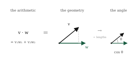
The three concepts below are all direct consequences of this single bridge.
It contains length. Take the dot product of a vector with itself. Every slot multiplies by itself, giving \(v_1^2 + v_2^2 + \cdots\). This is exactly what sat under the square root when we measured length. So
\[ \mathbf{v} \cdot \mathbf{v} = \lVert \mathbf{v} \rVert^2. \]
The dot product of a vector with itself is its length squared. Length is just the dot product applied to a matching pair.
It contains the angle. This relates the arithmetic back to our visual shadow:
\[ \mathbf{v} \cdot \mathbf{w} = \lVert \mathbf{v} \rVert \, \lVert \mathbf{w} \rVert \cos\theta, \]
Here, \(\theta\) is the angle between the arrows. The dot product contains the angle through \(\cos\theta\), but it is tangled together with both lengths. We will not prove this from scratch right now. The derivation is in the appendix for anyone who wants it. The most important skill is learning how to read the result.
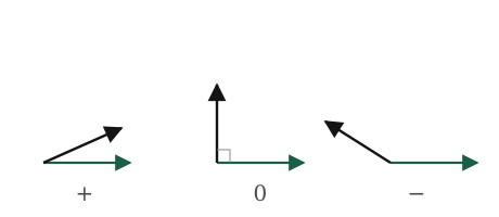
When the arrows perfectly align, \(\theta\) is zero and \(\cos\theta\) is one. The dot product is simply the two lengths multiplied together. At a right angle, \(\cos\theta\) is zero, and the whole calculation collapses to zero regardless of arrow length. Pointing opposite ways, \(\cos\theta\) is \(-1\), and the dot product becomes fully negative. The mathematical sign carries the summary. Positive means they lean together, zero means perpendicular, and negative means they lean apart.
It contains a test for right angles. This middle case is the one we will use the most. Two vectors are perpendicular exactly when their dot product is zero:
\[ \mathbf{v} \cdot \mathbf{w} = 0 \quad \Longleftrightarrow \quad \mathbf{v} \text{ and } \mathbf{w} \text{ are perpendicular.} \]
You do not need to measure any angles. You just multiply the slots and add them. If the answer is zero, the arrows stand at a perfect right angle. It is the cleanest test in linear algebra, and it comes directly from our basic arithmetic.
The dot product is just a sum of matching products. This is incredibly fast to write in NumPy.
Start with two vectors and form the calculation manually. Multiply matching slots and then add:
import numpy as np
v = np.array([2.0, 1.0])
w = np.array([1.0, 3.0])
products = v * w
print(products)
print(np.sum(products))[2. 3.]
5.0The v * w command multiplies slot by slot to give [2.0, 3.0]. Summing those gives 5.0. This is \(2\cdot1 + 1\cdot3\), performing the dot product in two clear steps. NumPy also handles this entirely in one built-in function:
print(np.dot(v, w))5.0It outputs the same 5.0. The np.dot function multiplies the matching slots and adds them, completely matching our manual steps.
Now we can confirm the three mathematical properties in code.
Length. The dot product of a vector with itself should equal its length squared:
print(np.dot(v, v))
print(np.linalg.norm(v) ** 2)
5.0
5.000000000000001Both return 5.0. The self-dot product and the squared length match perfectly.
The right-angle test. Two perpendicular vectors should give a dot product of zero. We will use \([1, 0]\) and \([0, 1]\), which point directly along the main axes:
a = np.array([1.0, 0.0])
b = np.array([0.0, 1.0])
print(np.dot(a, b))0.0The result is exactly zero. The simple arithmetic found the right angle completely on its own.
The angle. We can run the equation backwards to extract the pure angle. Since \(\mathbf{v} \cdot \mathbf{w} = \lVert \mathbf{v} \rVert \lVert \mathbf{w} \rVert \cos\theta\), we divide the dot product by the two lengths to isolate \(\cos\theta\). Then we use an inverse cosine function:
cos_theta = np.dot(v, w) / (np.linalg.norm(v) * np.linalg.norm(w))
theta = np.arccos(cos_theta)

print(cos_theta)
print(np.degrees(theta))
0.7071067811865475
45.00000000000001The angle between \(\mathbf{v}\) and \(\mathbf{w}\) calculates to about 45 degrees. Dividing by the lengths stripped away the scale of the arrows, leaving \(\cos\theta\) isolated. Separating the angle from the lengths only takes three lines of basic code.
None of this depends on the vectors being short lists. The dot product works flawlessly on three hundred numbers, and all three properties survive. np.dot still sums the products, the self-dot is still the length squared, and the zero test still finds a right angle. The single operation carries our entire toolkit into spaces we cannot see.
We can finally answer our opening question. How does a machine know two songs are similar? It takes their vectors, computes the dot product, and divides out the two physical lengths. The final result is \(\cos\theta\), a single number between \(-1\) and \(1\) that explains how perfectly the arrows align. A score close to \(1\) means they are nearly aligned. Close to \(0\) means unrelated. Below zero means opposite. This number is called cosine similarity.
\[ \text{cosine similarity} = \frac{\mathbf{v} \cdot \mathbf{w}}{\lVert \mathbf{v} \rVert \, \lVert \mathbf{w} \rVert} = \cos\theta \]
Dividing out the lengths is completely necessary. It is the reason cosine similarity is used instead of the raw dot product. Recall the loud song problem. A track with a high volume creates a long vector, and a raw dot product artificially rewards it just for being long. Stripping the lengths cancels that unwanted scale. Two songs count as similar only when they point the same way, regardless of volume. The angle provides the honest measurement.
This operation is how similarity is measured almost everywhere in machine learning.
Search engines run on it. Your query becomes a vector, and every document becomes a vector. The engine returns the documents that point most closely in the same direction as your query.
Recommendation systems run on it. Your personal taste is a vector, and every item is a vector. The system recommends whatever points your way.
Language models rely on it. When a model needs to find the correct text to answer a question, it turns both into vectors and ranks them by cosine similarity. A chatbot pulls the correct paragraph out of a long manual by rapidly computing thousands of dot products.
Attention mechanisms also run on it. When a model reads a sentence, it decides which words matter to each other. It gives every word a query vector and a key vector. It takes the dot product of one word’s query against every other word’s key. A large dot product signals that the words are highly relevant. This simple operation drives how a transformer model understands human language.
We also need to understand how this math can quietly fail. The dot product only represents similarity when the slots in both lists mean the exact same thing. If document vectors and query vectors use different rules, the dot product will confidently return a number, but that number is complete noise. If you break the shared meaning of the slots, the arithmetic keeps working while all logical value disappears. This is a very difficult bug to catch because the machine will never raise an error.
The dot product is easy to calculate but very easy to misread. Here are the most common misunderstandings to avoid.
The dot product is not basic vector multiplication. It is tempting to see \(\mathbf{v} \cdot \mathbf{w}\) as multiplying two vectors exactly like basic numbers. It is not, and the final output proves it. If you multiply two vectors slot by slot using v * w, you get an entirely new vector. The dot product takes that vector and adds its entries together, collapsing it into a single number. The dot product is multiplication followed immediately by addition. Writing v * w and np.dot(v, w) trigger two completely different operations.
A zero result does not mean unrelated in meaning. A zero dot product proves the arrows are geometrically perpendicular. It is easy to assume that perpendicular means the items have nothing to do with each other. These are completely different claims. Two word vectors might be perpendicular while still being deeply related in human meaning. The math only reports on the numerical geometry we built. Deciding if that geometry truly captures meaning is a separate challenge.
Stripping the lengths is not always the right choice. Cosine similarity divides out lengths to isolate the pure angle. This is great for songs or documents where raw length is just noisy interference. However, length is not always noise. Sometimes the physical magnitude of the data is extremely important. Throwing those lengths away destroys valuable information. Cosine similarity is only the right tool when direction is the only thing that carries meaning.
The inverse cosine function can fail silently. Recovering an angle by calling arccos can introduce a subtle calculation bug. In perfect mathematics, \(\cos\theta\) always stays securely between \(-1\) and \(1\). However, computer processors use floating-point approximations. The numbers can occasionally drift slightly outside that range due to tiny rounding errors. If you scale a vector to a perfect length of one and calculate its self-dot product, the machine might return a fraction just slightly over the limit:
import numpy as np

u = np.array([1.0, 1.0, 1.0])
u = u / np.linalg.norm(u)

cos_theta = np.dot(u, u)
print(cos_theta)1.0000000000000002Feeding a value larger than one to the arccos function causes a silent failure. It will not raise a formal error. Instead, it returns nan, which stands for not-a-number. This broken value poisons all calculations downstream:
print(np.arccos(cos_theta))nan/tmp/ipykernel_53807/2307936210.py:1: RuntimeWarning: invalid value encountered in arccos
print(np.arccos(cos_theta))The standard defense is to clip the value safely back into range before taking the inverse cosine:
theta = np.arccos(np.clip(cos_theta, -1.0, 1.0))
print(np.degrees(theta))0.0Clipping forces the tiny decimal error back to exactly one. The final angle correctly computes as zero. Always use np.clip when processing computed cosine values.
Try to solve these problems before expanding the answers. These require applying the concepts rather than reciting formulas.
1. Compute \(\mathbf{v} \cdot \mathbf{w}\) for \(\mathbf{v} = [3, 0]\) and \(\mathbf{w} = [0, 5]\). What does the answer tell you about the angle between them, without computing the angle?
2. Two vectors have a positive dot product. Then we replace \(\mathbf{w}\) with \(-\mathbf{w}\). What is the sign of the new dot product, and what has happened to the angle?
3. We have \(\mathbf{v} = [1, 1]\) and \(\mathbf{w} = [3, 3]\). Compute the dot product, and compute the cosine similarity. Why is one of these large and the other exactly \(1\)?
4. Without computing anything, which pair is more similar in direction: two vectors with a dot product of \(50\), or two vectors with a dot product of \(10\)?
5. A vector’s dot product with itself is \(0\). What can you say about the vector?
1. The dot product is \(3\cdot0 + 0\cdot5 = 0\). A zero result means the arrows are perpendicular. We know they sit at a right angle without directly measuring it. This matches the visual geometry, as the two vectors sit perfectly flat on the horizontal and vertical axes.
2. Flipping the vector negates every slot, so the dot product flips from positive to negative. Reversing the vector swings it to point in the opposite direction. This opens the angle past a right angle, turning an acute angle into an obtuse one.
3. The dot product is \(1\cdot3 + 1\cdot3 = 6\). The cosine similarity divides that by the two lengths. The lengths are \(\sqrt{2}\) and \(\sqrt{18}\), making the final similarity exactly \(1\). The raw dot product is artificially inflated because the second vector is physically long. Cosine similarity strips away that length to report on the pure direction. Because the second vector is just a scaled copy of the first, they point in exactly the same direction.
4. You cannot answer this question. The raw dot product mixes the angle together with the physical lengths. A score of \(50\) might come from two barely aligned but massive vectors. A score of \(10\) might come from two incredibly short vectors that point the exact same way. Without dividing out the lengths, the raw number cannot accurately rank similarity.
5. The dot product of a vector with itself is its length squared. If that result is zero, the vector has a length of exactly zero. The only vector with a zero length is an empty zero vector. It is a mathematical dot with no direction at all.